library(dplyr)
library(readr)More tidyverse practice
In this chapter we will introduce new (and reinforce already familiar) tidyverse concepts on another real-world data set, related to the metadata we looked previously. We will build the components of a processing and filtering (and in the next session, visualization) pipeline for a new Identity-by-Descent (IBD) data set that I recently got my hands on. We will proceed step by step, developing new components to the processing and analytical pipeline and learning how tidyverse can be useful in a very practical way, before we learn how to wrap it all up in a nice, structured, reproducible way in later parts of our workshop.
This is a real world example! You will be retracing the steps I had to work through in my job in August 2025 where I got sent a completely unfamiliar new data set of IBD segments and asked to do some science with it.
Why do this tidyverse stuff again? We just did this with the metadata table.
A few reasons:
The metadata is straightforward, easy to understand by looking at it. The IBD segment data (you will see) contains millions of data points. Being able to look at the data with your own eyes makes translating concepts to tidyverse operations much easier, which is why the metadata was a better starting point.
However, the metadata is just that, metadata. It’s a collection of meta information about individuals. But it’s not data you can do (biological) science with. As such, it’s much less exciting to really dig into more interesting concepts.
Related to point 2. above — the fact that the IBD data is more complex makes it more interesting to learn visualization on, like ggplot2 in the next section. So the rest of this session is a preparation for that.
The previous chapter on IBD basics was really about fundamental application of the most important tidyverse functions. This sesson is much more of a set of “recipes” that you should be able to apply to your own data, regardless of what statistics or biological measures you end up working with in your projects.
Again, here is how the start of our solutions script for this session will look like. Same as before:
Tip on doing interactive data science
Remember that the best way can solve any R problem is by building up a solution one little step at a time. First work in the R console, try bits and pieces of code interactively, and only when you’re sure you understand the problem (and solution) you can finalize it by writing it in your solution script (often saving the result in a variable for later use).
This helps a huge deal to avoid feeling overwhelmed by what can initially seem like a problem that’s too hard!
Let’s also read in data which we will be using in these exercises. These are coordinates of identity-by-descent (IBD) segments between pairs of individuals in a huge aDNA study we’ve already talked about. This data is big and quite complex — I prefiltered it to contain only IBD segments for chromosome 21. The IBD data should correspond to individuals in the metadata we worked with in the previous session.
ibd_segments <- read_tsv("https://tinyurl.com/simgen-ibd-segments")Rows: 461858 Columns: 6
── Column specification ────────────────────────────────────────────────────────
Delimiter: "\t"
chr (3): sample1, sample2, rel
dbl (3): chrom, start, end
ℹ Use `spec()` to retrieve the full column specification for this data.
ℹ Specify the column types or set `show_col_types = FALSE` to quiet this message.And we also need to read the corresponding metadata, with which you are already very closely familiar with:
metadata_all <- read_tsv("https://tinyurl.com/simgen-metadata")Rows: 4072 Columns: 24
── Column specification ────────────────────────────────────────────────────────
Delimiter: "\t"
chr (16): sampleId, popId, site, country, region, continent, groupLabel, gro...
dbl (8): latitude, longitude, age14C, ageHigh, ageLow, ageAverage, coverage...
ℹ Use `spec()` to retrieve the full column specification for this data.
ℹ Specify the column types or set `show_col_types = FALSE` to quiet this message.Note: I call it metadata_all because later we will be working with a smaller section of it, for more clarity. Therefore, metadata_all will be the original, unprocessed data set. It’s often very useful to keep raw data in our session like this.
Create a new R script in RStudio, (File -> New file -> R Script) and save it somewhere on your computer as tidy-advanced.R (File -> Save). Copy the chunks of code above into it (the library() and read_tsv() commands and let’s get started)!
Real world story
So, the story is that you just got a new data set from a bioinformatics software, in this case the IBDseq software for detecting IBD segments between pairs of individuals. Before you proceed with doing any kind of statistical analysis you need to do two things:
Exploring the data to see what is it that you just got. Never trust the data you’ve been given blindly and always do many sanity checks! In the process, you will gain more confidence in it, and also learn its ins and outs, which will be useful either way.
Filtering and processing it in a way which will make your work easier.
Let’s tackle step 1 first.
Exercise 1: Exploring new data
Again, the first step is always to familiarize yourself with the basic structure of the data. Which columns does the IBD data have? What’s the format of the data? What ranges or distributions of columns’ values do you have, and with what data types? Do you have information for the entire genome (all chromosomes)?
Hint: head(), colnames(), glimpse(), str(), table(), summary() which are either applicable to an entire data frame, or a specific column (column vectors can be extracted with the $ operator, of course).
As a sanity check, find out if you have metadata information for every individual in the sample1 and sample2 columns of the IBD table. What about the other way around – do all individuals in the metadata have some IBD relationship to another individual in the IBD segments table? If not, find out which individuals are these.
This is another sort of sanity checking you will be doing all the time. We can only analyze data for which we have metadata information (population assignment, geographical location, dating information), so let’s make sure we have what we need.
Hint: Another way to phrase this question is this: does every sample that appears in either sample1 or sample2 column of ibd_segments have a corresponding row in the sampleId column of metadata_all? Note that you can use the function unique() to get all values unique in a given vector (i.e., unique(ibd_segments$sample1) gives all individuals in the sample1 column, which has otherwise many duplicated entries). And remember the existence of the all() function, and the %in% operator, which can check if unique(ibd_segments$sample1) is in metadata_all$sampleId.
Hint: If this still doesn’t make sense, please work through my solution directly and try to understand it bit by bit! This is a bit more advanced than our previous tidyverse exercises.
With the basic sanity check above, we can be sure that our IBD segments table can be co-analyzed with the information in the metadata and that we won’t be missing anything important.
Exercise 2: IBD processing
Add a new column length to the ibd_segments data frame using the mutate() function, which will contain the length of each IBD segment in centimorgans (end - start). Save the data frame that mutate() returns back to the variable ibd_segments.
Note: Sometimes saving new things to already-defined variables leads to very messy code and its cleaner to create new variables for nex results. In this instance, we’re basically building up a processing pipeline whose purpose is to filter / mutate / clean a data frame for downstream use. In fact, later we will add individual steps of this pipeline name in several subsequent steps.
Exercise 3: Metadata processing
We have read our IBD table and added a new useful column length to it, so let’s proceed with the metadata. You already became familiar with it in the previous session—the goal here now is to transform it to a form more useful for downstream data co-analysis with the genomic IBD data.
Think of it this way: metadata contains all relevant variables for each individual in our data (age, location, population, country, etc.). IBD contains only genomic information. We eventually need to merge those two sets of information together to ask questions about population history and biology.
First, there’s much more information than we need for now, just take a look again:
colnames(metadata_all) [1] "sampleId" "popId" "site" "country" "region"
[6] "continent" "groupLabel" "groupAge" "flag" "latitude"
[11] "longitude" "dataSource" "age14C" "ageHigh" "ageLow"
[16] "ageAverage" "datingSource" "coverage" "sex" "hgMT"
[21] "gpAvg" "ageRaw" "hgYMajor" "hgYMinor" Realistically, given that our interest here is pairwise IBD segments, a lot of this metadata information is quite useless at this stage. Let’s make the data a bit smaller and easier to look at at a glance.
Use select() a subset of the metadata with the following columns and store it in a new variable metadata (not back to metadata_all! we don’t want to overwrite the original big table metadata_all in case we need to refer to it a bit later): sampleId, country, continent, ageAverage. Then rename sampleId to sample, popId to pop, and ageAverage to age just to save ourselves some typing later.
Just as you did in the previous chapter, use mutate() and if_else() inside the mutate() call to make sure that the “modern” individuals have the age set to 0, instead of NA (and everyone else’s age stays the same). In other words, for rows where age is NA, replace that NA with 0. Yes, you did this before, but try not to copy-paste your solution. Try doing this on your own first.
Hint: Remember the is.na() bit we used before! Try it on the age column vector if you need a reminder: is.na(metadata$age).
Our analyses will exclusively focus on modern humans. Filter out the three archaics in the metadata, saving the results into the same metadata variable again. As a reminder, these are individuals whose sample name is among c("Vindija33.19", "AltaiNeandertal", "Denisova") which you can test in a filter() command using the %in% operator.
Hint: Remember that you can get a TRUE / FALSE indexing vector (remember our R bootcamp session!) by not only column %in% c(... some values...) but you can also do the opposite test as !column %in% c(... some values...) (notice the ! operator in the second bit of code).
Experiment with the filter() command in your R console first if you want to check that your filtering result is correct.
Status of our data so far
We now have a cleaner IBD table looking like this:
head(ibd_segments)# A tibble: 6 × 7
sample1 sample2 chrom start end rel length
<chr> <chr> <dbl> <dbl> <dbl> <chr> <dbl>
1 VK548 NA20502 21 58.3 62.1 none 3.75
2 VK528 HG01527 21 24.8 27.9 none 3.04
3 PL_N28 NEO36 21 14.0 16.5 none 2.44
4 NEO556 HG02230 21 13.1 14.0 none 0.962
5 HG02399 HG04062 21 18.8 21.0 none 2.21
6 EKA1 NEO220 21 30.1 35.8 none 5.72 And here’s our metadata information:
head(metadata)# A tibble: 6 × 4
sample country continent age
<chr> <chr> <chr> <dbl>
1 NA18486 Nigeria Africa 0
2 NA18488 Nigeria Africa 0
3 NA18489 Nigeria Africa 0
4 NA18498 Nigeria Africa 0
5 NA18499 Nigeria Africa 0
6 NA18501 Nigeria Africa 0In our original metadata_all table we have the groupAge column with these values:
table(metadata_all$groupAge)
Ancient Archaic  Modern
   1664       3    2405
Note that in the new metadata we removed it because it’s not actually useful for most data analysis purposes (it has only three values). For instance, later we might want to do some fancier analyses, looking at IBD as a time series, not just across basically two temporal categories, “young” and “old”.
To this end, let’s create more useful time-bin categories! This will require a bit more code than above solutions. Don’t feel overwhelmed! I will first introduce a useful function using a couple of examples for you to play around with in your R console. Only then we will move on to an exercise in which you will try to implement this on the full metadata table! For now, keep on reading and experimenting in your R console!
It will be worth it, because this kind of binning is something we do all the time in computational biology, in every project.
Let’s introduce an incredibly useful function called cut(). Take a look at ?cut help page and skim through it to figure out what it does. As a bit of a hint, we will want to add a new metadata column which will indicate in which age bin (maybe, split in steps of 5000 years) do our individuals belong to.
Here’s a small example to help us get started. Let’s pretend for a moment that the df variable created below is a example representative of our full-scale big metadata table. Copy this into your script, so that you can experiment with the cut() technique in this section.
# a toy example data frame mimicking the age column in our huge metadata table
df <- data.frame(
  sample = c("a", "b", "c", "d", "x", "y", "z", "q", "w", "e", "r", "t"),
  age = c(0, 0, 1000, 0, 5000, 10000, 7000, 13000, 18000, 21000, 27000, 30000)
)
df
sample age
1 a 0
2 b 0
3 c 1000
4 d 0
5 x 5000
6 y 10000
7 z 7000
8 q 13000
9 w 18000
10 e 21000
11 r 27000
12 t 30000Let’s do the time-binning now! Think about what the cut() function does here based on the result it gives you on the little example code below. You can pretend for now that the ages variable corresponds to age of our samples in the huge metadata table. Again, try running this on your own to see what happens when you run this code in your R console. Particularly, take a look at the format of the new column age_bin:
# let's first generate the breakpoints for our bins (check out `?seq` if
# you're confused by this!)
breakpoints <- seq(0, 50000, by = 5000)
# take a look at the breakpoints defined:
breakpoints
##  [1]     0  5000 10000 15000 20000 25000 30000 35000 40000 45000 50000

# create a new column of the data frame, containing bins of age using our breakpoints
df$age_bin <- cut(df$age, breaks = breakpoints)
# take a look at the data frame (with the new column `age_bin` added)
df
##    sample   age         age_bin
## 1       a     0            <NA>
## 2       b     0            <NA>
## 3       c  1000       (0,5e+03]
## 4       d     0            <NA>
## 5       x  5000       (0,5e+03]
## 6       y 10000   (5e+03,1e+04]
## 7       z  7000   (5e+03,1e+04]
## 8       q 13000 (1e+04,1.5e+04]
## 9       w 18000 (1.5e+04,2e+04]
## 10      e 21000 (2e+04,2.5e+04]
## 11      r 27000 (2.5e+04,3e+04]
## 12      t 30000 (2.5e+04,3e+04]
The function cut() is extremely useful whenever you want to discretize some continuous variable in bins (basically, a little similar to what a histogram does in context of plotting). Doing statistics on this kind of binned data is something we do very often. So never forget that cut() is there to help you! For example, you could also use the same concept to partition samples into categories based on “low coverage”, “medium coverage”, “high coverage”, etc.
In the example of the cut() function right above, what is the data type of the column age_bin created by the cut() function? Use glimpse(df) to see this data type, then skim through the documentation of ?factor. What is a “factor” according to this documentation?
Note: This is a challenging topic. Please don’t stress. When we’re done I’ll walk through everything myself, interactively, and will explain things in detail. Take this information on “factors” as something to be aware of and a concept to be introduced to, but not something to necessarily be an expert on!
Having learned about ?factor above, consider the two following vectors and use them for experimentation when coming up with answers. What do you see when you print them out in your R console (by typing x1 and x2)? And what happens when you apply the typeof() function on both of them? x2 gives you a strange result — why? What do you get when you run the following command levels(x2)? What do you get when you run as.character(x2)?
x1 <- c("hello", "hello", "these", "are", "characters/strings")
x2 <- factor(x1)
In applying cut() to the toy data frame df, why is the age_bin value equal to NA for some of the rows?
Note: The discussion of “factors” should’ve been technically part of our R bootcamp chapter, on the topic of “data types”. However, that section was already too technical, so I decided to move it here to the data analysis section, because I think it makes more sense to explain it in a wider context.
The scientific notation format of bin labels with 5+e3 etc. is very annoying to look at. How can you use the dig.lab = argument of the cut() functions to make this prettier? Experiment in the R console to figure this out, then modify the df$age_bin <- cut(df$age, breaks = breakpoints) command in your script accordingly.
You have now learned that cut() has an optional argument called include.lowest =, which includes the lowest value of 0 (representing the “present-day” age of our samples) in the lowest bin [0, 5]. However, in the case of our assignment of samples from present-day, this is not what we want. We want present-day individuals to have their own category called “present-day”.
Here’s a useful bit of code I use often for this exact purpose, represented as a complete self-contained chunk of the time-binning code. If we start from the original toy example data frame (with the NA values assigned to present-day ages of 0):
df sample age age_bin
1 a 0 <NA>
2 b 0 <NA>
3 c 1000 (0,5000]
4 d 0 <NA>
5 x 5000 (0,5000]
6 y 10000 (5000,10000]
7 z 7000 (5000,10000]
8 q 13000 (10000,15000]
9 w 18000 (15000,20000]
10 e 21000 (20000,25000]
11 r 27000 (25000,30000]
12 t 30000 (25000,30000]We can fix this by the following three-step process, described in the comments. Don’t stress about any of this! Just run this code on your own and try to relate the # text description of each step in comments to the code itself. Every thing that’s being done here are bits and pieces introduced above.
# 0. assign each row to a bin based on given breakpoints
df$age_bin <- cut(df$age, breaks = breakpoints, dig.lab = 10)

# 1. extract labels (no "present-day" category yet)
bin_levels <- levels(df$age_bin)

df <-
  df %>%
  mutate(
    age_bin = as.character(age_bin),  # 2. convert factors back to "plain strings"
    age_bin = if_else(is.na(age_bin), "present-day", age_bin), # 3. replace NA with "present-day",
    age_bin = factor(age_bin, levels = c("present-day", bin_levels)) # 4. convert to factor (to maintain order of levels)
  )
Please run the code above bit by bit, inspecting the variables you create (or modify) after each step. Remember the CTRL / CMD + Enter shortcut for stepping through code!
When we print the modified df table, we see all bins properly assigned now, including the present-day samples with ages at 0:
df sample age age_bin
1 a 0 present-day
2 b 0 present-day
3 c 1000 (0,5000]
4 d 0 present-day
5 x 5000 (0,5000]
6 y 10000 (5000,10000]
7 z 7000 (5000,10000]
8 q 13000 (10000,15000]
9 w 18000 (15000,20000]
10 e 21000 (20000,25000]
11 r 27000 (25000,30000]
12 t 30000 (25000,30000]This is a very useful pattern which you will get to practice now on the full metadata table, by literally applying the same code on the big table.
Now that you’re familiar with the cut() technique for binning values, use the functions mutate() and cut() again (in exactly the same way as we did on the df table in the code chunk above!) to create a new column age_bin this time on the whole metadata table. The new column should carry a category age of each individual in steps of 10000 years again.
Hint: As we did above, first assign the age_bin column using the cut() function, then modify the column accordingly with the mutate() snippet to set “present-day” in the age_bin for all present-day individuals.
How many individuals did we end up with in each age_bin? Use table() to answer this question (and also to sanity check your final results), to make sure everything worked correctly.
Recipe for merging metadata
After basic processing and filtering of the primary data (in our case, the genomic coordinates of pairwise IBD segments), we often need to annotate this data with some meta information… which is what we already processed too! What does this mean? Take a look at our IBD data in its current state again:
head(ibd_segments)# A tibble: 6 × 7
sample1 sample2 chrom start end rel length
<chr> <chr> <dbl> <dbl> <dbl> <chr> <dbl>
1 VK548 NA20502 21 58.3 62.1 none 3.75
2 VK528 HG01527 21 24.8 27.9 none 3.04
3 PL_N28 NEO36 21 14.0 16.5 none 2.44
4 NEO556 HG02230 21 13.1 14.0 none 0.962
5 HG02399 HG04062 21 18.8 21.0 none 2.21
6 EKA1 NEO220 21 30.1 35.8 none 5.72 When we analyze things down the line, we might want to look at IBD patterns over space and time, look at some temporal changes, etc. However, our IBD data has none of the information in it! Besides names of individuals (from which population, at which time, which geographical location?) we have nothing, so even if we were to do run our friends group_by() and summarize() to get some summary statistics to get some insights into the history or biological relationships between our samples, we have no idea to correlate them to other variables… precisely because those variables are elsewhere in a completely different table we called metadata.
We now need to put both sources of information into a single joint format. I call this “metadata merging”, and it is something we always want to do regardless of what kinds of statistics or measures we work with.
The technique below is again a very useful recipe for your future work.
Again, the annotation that we need is in the metadata table — it has information about ages and geography:
head(metadata)# A tibble: 6 × 5
sample country continent age age_bin
<chr> <chr> <chr> <dbl> <fct>
1 NA18486 Nigeria Africa 0 present-day
2 NA18488 Nigeria Africa 0 present-day
3 NA18489 Nigeria Africa 0 present-day
4 NA18498 Nigeria Africa 0 present-day
5 NA18499 Nigeria Africa 0 present-day
6 NA18501 Nigeria Africa 0 present-dayWhat we need to do is join our IBD data with a selection of the most important variables in our metadata, which is what we’re going to do now.
This bit might be a bit frustrating and repetitive if I made this into an exercise for you, so just inspect the following code, run it yourself (and put it into your own script) and try to make sense of it. Take this as a recipe that you can modify and reuse in your own projects later!
I’m happy to answer questions!
Step 1.
For each IBD segment (a row in our table ibd_segments) we have two individuals on each row, sample1 and sample2. Therefore, we will need to annotate each row of the ibd_segments table with metadata information for both individuals. Let’s start by making a copy of the metadata table, caling those copies metadata1 and metadata2:
metadata1 <- metadata
metadata2 <- metadata
Step 2.
The columns of these metadata copies are the same, which you can verify by running this:
colnames(metadata1)
## [1] "sample"    "country"   "continent" "age"       "age_bin"
head(metadata1, 1)
## # A tibble: 1 × 5
##   sample  country continent   age age_bin
##   <chr>   <chr>   <chr>     <dbl> <fct>
## 1 NA18486 Nigeria Africa 0 present-daycolnames(metadata2)
## [1] "sample" "country" "continent" "age" "age_bin"
head(metadata2, 1)
## # A tibble: 1 × 5
## sample country continent age age_bin
## <chr> <chr> <chr> <dbl> <fct>
## 1 NA18486 Nigeria Africa 0 present-dayObviously this doesn’t work if we want to refer to a location of sample1 or sample2, respectively. Here’s another useful trick for this. Observe what paste0() function does in this situation:
# original columns
colnames(metadata1)
[1] "sample" "country" "continent" "age" "age_bin" # columns with a number added after
paste0(colnames(metadata1), "1")[1] "sample1" "country1" "continent1" "age1" "age_bin1" So using paste0() we can append “1” or “2” to each column name of both tables. We can use the same approach to assign new columns to both of our metadata copies:
colnames(metadata1) <- paste0(colnames(metadata1), "1")
colnames(metadata2) <- paste0(colnames(metadata2), "2")
Now we have both metadata tables with columns renamed. Let’s check this to make sure we did this correctly:
colnames(metadata1)[1] "sample1" "country1" "continent1" "age1" "age_bin1" colnames(metadata2)[1] "sample2" "country2" "continent2" "age2" "age_bin2" Step 3.
Now we are ready to join the table of IBD segments.
The final piece of the puzzle is a JOIN operation from the realm of computer databases. A rather complex topic, which can be interpreted very easily in our situation, and can be schematically described by the following diagram of a so-called “inner join”, implemented in dplyr by a function inner_join():
Note: If you’re more familiar with tidyverse from before, I still think joins might be a relatively new topic. If so, please take a bit of time to read the dplyr documentation on join operations. Joins are a superpower of data science.
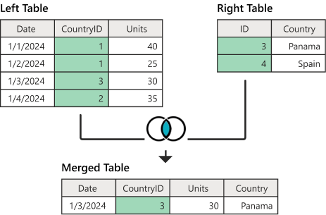
What this operation does is that it creates a “merged” table, consisting of the columns of both “left” and “right” tables, where the “merged” table rows consist of such rows from “left” and “right”, where the two tables have a matching “key” column (here highlighted in green). Just take a moment and try to trace the one row of the “merged” table at the bottom of the diagram to the row(s) of the “left” and “right” tables based on the value of the green key column in both of them.
Now, consider the columns of our three tables now:
ibd_segmentscolumns:
[1] "sample1" "sample2" "chrom" "start" "end" "rel" "length" metadata1andmetadata2columns:
[1] "sample1" "country1" "continent1" "age1" "age_bin1" [1] "sample2" "country2" "continent2" "age2" "age_bin2" Here’s what happens when you perform an inner join like this (note that we specify by what column should we be merging, effectively saying which column is the key corresponding to the green column in the diagram above):
ibd_merged <- inner_join(ibd_segments, metadata1, by = "sample1")Take a look at the results, saved in a new variable ibd_merged, by typing it into your R console. Our IBD table now has added metadata information for individuals in column sample1, awesome! We can verify this by listing all column names:
# original IBD table:
head(ibd_segments, n = 3)
# A tibble: 3 × 7
sample1 sample2 chrom start end rel length
<chr> <chr> <dbl> <dbl> <dbl> <chr> <dbl>
1 VK548 NA20502 21 58.3 62.1 none 3.75
2 VK528 HG01527 21 24.8 27.9 none 3.04
3 PL_N28 NEO36 21 14.0 16.5 none 2.44# IBD table with metadata1 merged in:
head(ibd_merged, n = 3)# A tibble: 3 × 11
sample1 sample2 chrom start end rel length country1 continent1 age1
<chr> <chr> <dbl> <dbl> <dbl> <chr> <dbl> <chr> <chr> <dbl>
1 VK548 NA20502 21 58.3 62.1 none 3.75 Norway Europe 1000
2 VK528 HG01527 21 24.8 27.9 none 3.04 Norway Europe 1050
3 PL_N28 NEO36 21 14.0 16.5 none 2.44 Poland Europe 6074.
# ℹ 1 more variable: age_bin1 <fct>How do we add metadata for the second sample? We do it in the same way, except now we join in the second table (and we save the results back to the new variable ibd_merged, to be able to compare the differences):
ibd_merged <- inner_join(ibd_merged, metadata2, by = "sample2")In fact, I do this so often for basically every computational biology project, that I like to use this concise bit of code to do it all in one go (this is what you should add to your script!):
ibd_merged <-
  ibd_segments %>%                          # 1. primary data without metadata
  inner_join(metadata1, by = "sample1") %>% # 2. add metadata for sample1
  inner_join(metadata2, by = "sample2")     # 3. add metadata for sample2
Again, we can verify that our new table has metadata columns for both sample1 and sample2:
head(ibd_segments, n = 3)# A tibble: 3 × 7
sample1 sample2 chrom start end rel length
<chr> <chr> <dbl> <dbl> <dbl> <chr> <dbl>
1 VK548 NA20502 21 58.3 62.1 none 3.75
2 VK528 HG01527 21 24.8 27.9 none 3.04
3 PL_N28 NEO36 21 14.0 16.5 none 2.44head(ibd_merged, n = 3)# A tibble: 3 × 15
sample1 sample2 chrom start end rel length country1 continent1 age1
<chr> <chr> <dbl> <dbl> <dbl> <chr> <dbl> <chr> <chr> <dbl>
1 VK548 NA20502 21 58.3 62.1 none 3.75 Norway Europe 1000
2 VK528 HG01527 21 24.8 27.9 none 3.04 Norway Europe 1050
3 PL_N28 NEO36 21 14.0 16.5 none 2.44 Poland Europe 6074.
# ℹ 5 more variables: age_bin1 <fct>, country2 <chr>, continent2 <chr>,
# age2 <dbl>, age_bin2 <fct>And this concludes merging of the primary IBD data with all necessary meta information! Every computational project has something like this somewhere. Of course, in the case of your primary data which could be observations at particular ecological sampling sites or excavation sites, etc., this annotation might involve metadata with more specific geographical information, environmental data, etc. But the idea of using join for the annotation remains the same.
Exercise 4. Final data processing
You’ve already seen the super useful function paste() (and also paste0()) which useful whenever we need to join the elements of two (or more) character vectors together. The difference between them is that paste0() doesn’t add a space between the individual values and paste() does (the latter also allows you to customize the string which should be used for joining instead of the space).
Take a look at your (now almost finalized) table ibd_merged:
head(ibd_merged)# A tibble: 6 × 15
sample1 sample2 chrom start end rel length country1 continent1 age1
<chr> <chr> <dbl> <dbl> <dbl> <chr> <dbl> <chr> <chr> <dbl>
1 VK548 NA20502 21 58.3 62.1 none 3.75 Norway Europe 1000
2 VK528 HG01527 21 24.8 27.9 none 3.04 Norway Europe 1050
3 PL_N28 NEO36 21 14.0 16.5 none 2.44 Poland Europe 6074.
4 NEO556 HG02230 21 13.1 14.0 none 0.962 Russia Europe 7030
5 HG02399 HG04062 21 18.8 21.0 none 2.21 China Asia 0
6 EKA1 NEO220 21 30.1 35.8 none 5.72 Estonia Europe 4240
# ℹ 5 more variables: age_bin1 <fct>, country2 <chr>, continent2 <chr>,
# age2 <dbl>, age_bin2 <fct>When we get to comparing IBD patterns between countries, time bins, etc., it might be useful to have metadata columns specific for that purpose. What do I mean by this? For instance, consider these two vectors and the result of pasting them together. Having this combined pair information makes it very easy to cross-compare multiple sample categories together, rather than having to keep track of two variables v1 or v2, we have just the merged pairs:
v1 <- c("Denmark", "Czech Republic", "Estonia")
v2 <- c("Finland", "Italy", "Estonia")

pairs_v <- paste(v1, v2, sep = ":")
pairs_v
[1] "Denmark:Finland" "Czech Republic:Italy" "Estonia:Estonia" Let’s create this information for country1/2, continent1/2, and age_bin1/2 columns.
Specifically, use the same paste() trick in a mutate() function to add a new column to your ibd_merged table named country_pair, which will contain a vector of values created by joining of the columns country1 and country2. Add this column .before the chrom column for clearer visibility (check out ?mutate if you need a refresher on how does its .before = argument work). Then do the same to create a region_pair based on continent1 and continent2. Save the result back to the variable named ibd_merged.
Hint: Note that you can create multiple new columns with mutate(), but you can also pipe %>% one mutate() into another mutate() into another mutate(), etc.!
In addition to computing statistics across pairs of geographical regions, we will also probably want to look at temporal patterns. Create a new column time_pair, which will in this case contains a paste() combination of age_bin1 and age_bin2, added .after the region_pair column. Save the result back to the ibd_merged variable.
Exercise 5: Reproducibility intermezzo
You have written a lot of code in this chapter, both for filtering and processing of the IBD data and the metadata. Your script is already very long (and maybe messy—I organized things like this on purpose, so this isn’t on you!).
If you need to ever update or change something (which you always will during a project, usually many times over) it can be hard to figure out which line of your script should be modified. If you forget to update something somewhere in a long script, you’re in big trouble (and sometimes you won’t even find out where’s the problem until its too late).
Our session on reproducibility is in the following chapter, and will introduce various techniques towards making a project codebase tidyly structured and reproducible. But for now, let’s work towards making our current IBD pipeline a little bit more reusable (which we will leverage in the next session on ggplot2).
Create a new script called ibd_utils.R in your RStudio and create the following functions in that script (see the list below). Then copy-paste bits and pieces from your solutions above and add them to the bodies of these functions accordingly, so that each function contains all the code we used above for that particular step. (There are three functions, for each part of the pipeline code we developed in this session.)
If you’ve never written R functions before and are confused, don’t worry. You can skip ahead and use my solution directly (just paste that solution to your ibd_utils.R script)!
Yes, this is the first time I specifically told you that you can copy-paste something directly. :)
If you do, however, examine the code in each of the three functions, and try to make a connection between each function — line by line — and the code you ran earlier in our session! Because these functions really do contain all your code, just “modularized” in a reusable form. Refer back to the exercise on writing custom functions in our R basecamp session if you need a refresher on the R syntax used for this.
Here are the functions you should create:
First, don’t forget to load all packages needed using
library()calls at the top of theibd_utils.Rscript.Function
process_ibd <- function() { ... }which will:
- read the IBD data from the internet like you did above using
read_tsv() - process it in the same way you did above, adding the length column
- return the processed table with IBD segments in the same way like you produced the
ibd_segmentsdata frame withreturn(ibd_segments)at the last line of that function
- Function
process_metadata <- function(bin_step) { ... }, which will (accepting a singlebin_stepargument):
- download the metadata from the internet like you did above,
- process and filter it in the same way like above (replacing
NAinagecolumn, filtering out unwanted individuals, adding theage_bincolumn by binning according to thebin_stepfunction parameter, etc.) - return the processed table with this processed metadata in the same way like you produced the
metadatadata frame asreturn(metadata)
- Function
join_metadata <- function(ibd_segments, metdata) { ... }, which will accept two argumentsibd_segmentsandmetadata(produced by the two functions above) and then:
- join the
ibd_segmentstable with themetadatatable - add the three
country_pair,region_pair, andtime_paircolumns - return the finalized table with all information, just like you created your
ibd_mergedtable above, asreturn(ibd_merged)
Do not write all the code at once! Start with the first function, test it by executing it in your R console independently, checking that your results make sense before you move on to the other function! Building up more complex pipelines from simple components is absolutely critical to minimize bugs!
Make sure to add comments to your code! Reproducibility is only half of the story – you (and other people) need to be able to understand your code a long time after you wrote it.
Hint: If this looks overwhelming and scary, then remember that function is a block of code (optionally accepting arguments) which simply wraps in { and } the code already written by you above, and calls return on the result.
Hint: An extremely useful shortcut when writing R functions is “Run function definition” under Code -> Run region. Remember that keyboard shortcut! (On macOS it’s Option+CMD+F).
To summarize, basically fill in the following template:
After you’re done with the previous exercise, and are confident that your functions do what they should, create a new script (you can name it something like ibd_pipeline.R), save it to the same directory as your script ibd_utils.R, and add the following code to it, which, when you run it, will execute your entire pipeline and create the final ibd_merged table in a fully automated way. As a final test, restart your R session (Session -> Restart R) and run the script ibd_pipeline.R (you can use the => Run button in the top right corner of your editor panel).
You just build your (maybe first?) reproducible, automated data processing pipeline! 🎉
Note: The source() command executes all the code in your utility script and therefore makes your custom-built functions available in your R session. This is an incredibly useful trick which you should use all the time whenever you modularize your code into reproducible functions in their own scripts.
# you might need to change the path if your ibd_utils.R is in a different location
library(dplyr)
library(readr)

source("ibd_utils.R")

metadata <- process_metadata()
ibd_segments <- process_ibd(bin_step = 10000)

ibd_merged <- join_metadata(ibd_segments, metadata)
Downloading and processing metadata...Downloading and processing IBD data...Joining IBD data and metadata...Congratulations! You’ve just passed an important milestone of learning how to structure and modularize your code in a reproducible, efficient way!
This is not a joke and I really, really mean it. Most scientists are unfortunately never taught this important concept. Over the next sessions you will see how much difference does (admittedly very annoying!) setup makes, and even learn other techniques how to make your computational research more robust and reliable.
If this was too much programming and you struggled to push through, please don’t worry. As I said at the beginning, this session was mostly about showing you a useful recipe for processing data and to demonstrate why tidyverse is so powerful.
Taking a look at my solution again (now copied to your on ibd_utils.R script), and being able to understand the general process by reading the code line by line is enough at this stage.
Point your cursor somewhere inside the process_ibd() call in your new script ibd_pipeline.R and press CTRL + .. This is how easy it is to navigate code, even when we modularized it across multiple files!
“Take home exercise”
Take your own data and play around with it using the concepts you learned above. If the data isn’t in a form that’s readily readable as a table with something like read_tsv(), please talk to me! tidyverse is huge and there are packages for munging all kinds of data. I’m happy to help you out.
Don’t worry about “getting somewhere”. Playing and experimenting (and doing silly things) is the best way to learn.
For more inspiration on other things you could do with your data, take a look at the dplyr cheatsheet.
In each following session, you’ll have the opportunity to create beautiful publication-quality visualizations on your data using the ggplot2 package. So stay tuned!
Additional resources
If you’re more comfortable with tidyverse and breezed through this content quickly, here are some resources on topics I think you should study (and do exercises in them) to take your data science skills to the next level:
- A huge topic I wish I had a chance to get into here are transformations between long and wide table formats – link to a chapter of R4DS book, tidyr cheatsheet.
As an exercise, try to convert the various “age-related” columns in our metadata table (encoded in the “wide format”) to a long format after studying this chapter. Then learn how to transform the long format back into the wide format!
Regular expression are another critical topic which every professional data scientist should be familiar with – link to a chapter of R4DS book, regex cheatsheet.
Study the chapter on joins in more detail – link.
Look up some guidelines for modern R coding style – link.
Not entirely related to tidyverse but a critical component of large scale data analysis pipelines in R (all of which feature dplyr and others internally), particularly if they involve parallelized computing are futures. Especially the package furrr is an absolute pleasure to use – link.
A companion to furrr which focuses on elegant interface for non-paralellized iteration is called purrr – here is a very nice cheatsheet.