Spatial PCA

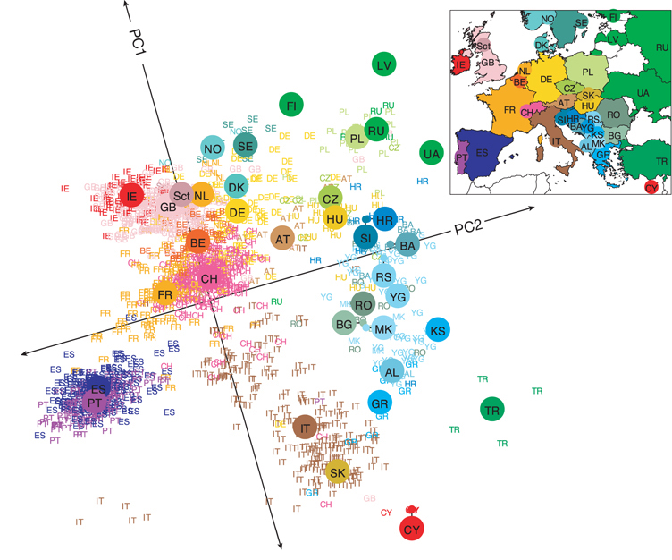
WIP: Exploring how (and when) PCA patterns recapitulate geographical history of populations, inspired by this figure by Novembre et al. (2008).

library(slendr)
init_env()

The interface to all required Python modules has been activated.

library(admixr)
library(cowplot)

source("popgen_files/popgen_utils.R")

model <- landscape_model(rate = 0.3, Ne = 10000)

# pdf("exercise5.pdf", width = 8, height = 5)
# for (n in c(50, 25, 10, 5, 2, 1)) {
  n <- 10
  schedule <- landscape_sampling(model, n)

  ts <- msprime(model, samples = schedule, sequence_length = 20e6, recombination_rate = 1e-8) %>% ts_mutate(1e-8)

  samples <- ts_samples(ts)

  ts_eigenstrat(ts, "popgen_files/spatial_pca1")

454 multiallelic sites (0.279% out of 162540 total) detected and removed

EIGENSTRAT object
=================
components:
  ind file: popgen_files/spatial_pca1.ind
  snp file: popgen_files/spatial_pca1.snp
  geno file: popgen_files/spatial_pca1.geno

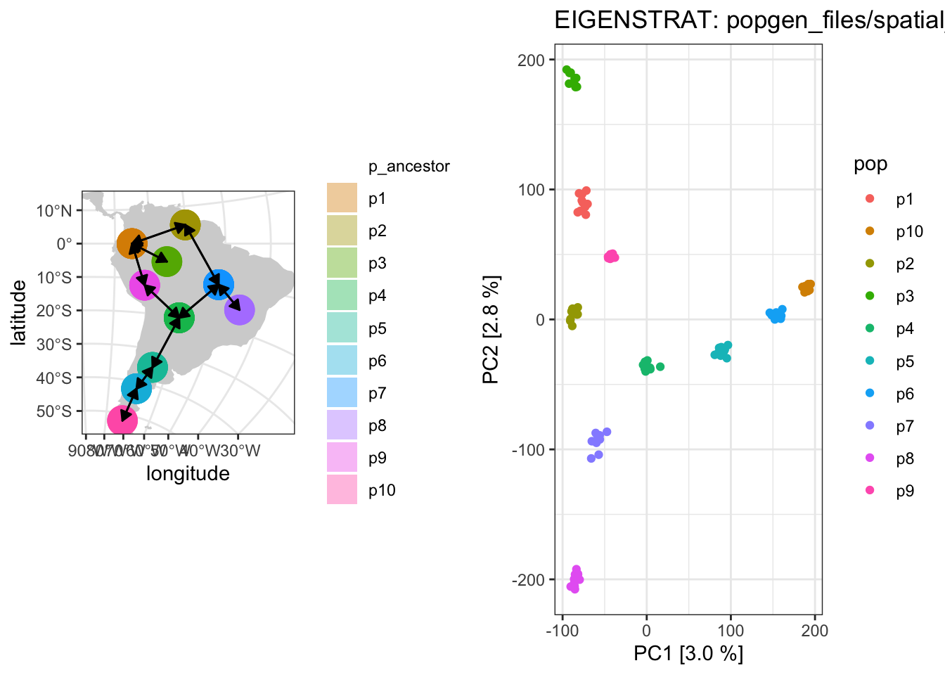
  plot_pca("popgen_files/spatial_pca1", ts, model = "map", color_by = "pop")

PCA cache for the given EIGENSTRAT data was not found. Generating it now (this might take a moment)...

Warning: Visualising population labels on a map requires a higher slendr
version

Warning: All gene-flow event will be visualized at once. If you wish to visualize
gene flows at a particular point in time, use the `time` argument.

Warning: Non-spatial populations in your model won't be visualized

# }
# dev.off()

Per-population Ne values

library(slendr)
init_env()

The interface to all required Python modules has been activated.

library(admixr)
library(cowplot)

source("popgen_files/popgen_utils.R")

Ne <- list(
  p1 = 10000,
  p2 = 10000,
  p3 = 10000,
  p4 = 10000,
  p5 = 100,
  p6 = 10000,
  p7 = 10000,
  p8 = 10000,
  p9 = 10000,
  p10 = 10000
)

model <- landscape_model(rate = 0.3, Ne = Ne)

n <- list(
  p1 = 50,
  p2 = 50,
  p3 = 50,
  p4 = 50,
  p5 = 5,
  p6 = 50,
  p7 = 50,
  p8 = 50,
  p9 = 50,
  p10 = 50
)

schedule <- landscape_sampling(model, n)

ts <- msprime(model, samples = schedule, sequence_length = 20e6, recombination_rate = 1e-8) %>% ts_mutate(1e-8)

ts_eigenstrat(ts, "popgen_files/spatial_pca2")

1076 multiallelic sites (0.427% out of 252247 total) detected and removed

EIGENSTRAT object
=================
components:
  ind file: popgen_files/spatial_pca2.ind
  snp file: popgen_files/spatial_pca2.snp
  geno file: popgen_files/spatial_pca2.geno

read_ind(eigenstrat("popgen_files/spatial_pca2"))

# A tibble: 455 × 3
   id    sex   label
   <chr> <chr> <chr>
 1 p1_1  U     p1_1 
 2 p1_2  U     p1_2 
 3 p1_3  U     p1_3 
 4 p1_4  U     p1_4 
 5 p1_5  U     p1_5 
 6 p1_6  U     p1_6 
 7 p1_7  U     p1_7 
 8 p1_8  U     p1_8 
 9 p1_9  U     p1_9 
10 p1_10 U     p1_10
# ℹ 445 more rows

ts_samples(ts)

# A tibble: 455 × 3
   name   time pop  
   <chr> <dbl> <chr>
 1 p1_1  10000 p1   
 2 p1_2  10000 p1   
 3 p1_3  10000 p1   
 4 p1_4  10000 p1   
 5 p1_5  10000 p1   
 6 p1_6  10000 p1   
 7 p1_7  10000 p1   
 8 p1_8  10000 p1   
 9 p1_9  10000 p1   
10 p1_10 10000 p1   
# ℹ 445 more rows

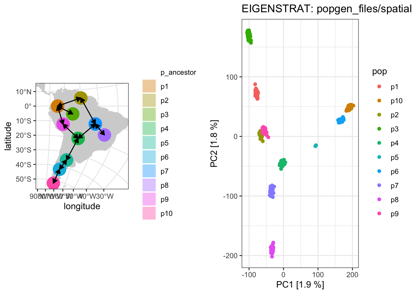
plot_pca("popgen_files/spatial_pca2", ts, model = "map", color = "pop")

PCA cache for the given EIGENSTRAT data was not found. Generating it now (this might take a moment)...

Warning: Visualising population labels on a map requires a higher slendr
version

Warning: All gene-flow event will be visualized at once. If you wish to visualize
gene flows at a particular point in time, use the `time` argument.

Warning: Non-spatial populations in your model won't be visualized