library(slendr)
init_env(quiet = TRUE)

chimp <- population("CHIMP", time = 7e6, N = 5000)
afr <- population("AFR", parent = chimp, time = 6e6, N = 15000)
eur <- population("EUR", parent = afr, time = 60e3, N = 3000)
nea <- population("NEA", parent = afr, time = 600e3, N = 1000, remove = 40e3)

gf <- gene_flow(from = nea, to = eur, rate = 0.03, start = 55000, end = 50000)

model <- compile_model(
  populations = list(chimp, nea, afr, eur),
  gene_flow = gf,
  generation_time = 30
)

# Here we scheduled the sampling of two Neanderthals at 70kya and 40kya
nea_samples <- schedule_sampling(model, times = c(70000, 40000), list(nea, 1))

# Here we schedule one Chimpanzee sample, 5 African samples, and 10 European samples
present_samples <- schedule_sampling(model, times = 0, list(chimp, 1), list(afr, 5), list(eur, 10))

# We also schedule the recording of one European sample between 50kya and 2kya,
# every 2000 years
times <- seq(40000, 2000, by = -2000)
emh_samples <- schedule_sampling(model, times, list(eur, 1))

# Because those functions produce nothing but a data frame, we can bind
# individual sampling schedules together
schedule <- rbind(nea_samples, present_samples, emh_samples)

# Simulate a tree sequence (with mutations) -- feel free to increase the amount
# of sequence from 20Mb to something like 100Mb (100e6 bp) if you want  to reduce
# the statistical noise a bit
ts <-
  msprime(model, sequence_length = 20e6, recombination_rate = 1e-8, samples = schedule, random_seed = 1269258439) %>%
  ts_mutate(mutation_rate = 1e-8, random_seed = 1269258439)

tsTree-sequence statistics
Introduction
In this session, you are going to build on top of the results from the previous session on programming demographic models. Specifically, you will learn how to compute population genetic statistics on slendr-simulated tree sequences using slendr’s interface to the tskit Python module.
Note: If you ever get totally stuck, take a look at the provided solution. The point of these exercises is to learn things, not fight through endless frustration. That said, try not to look at the solution automatically, always take a stab at solving each exercise on your own first. And when you do decide to look at my solution, always try to understand the code on your own, line by line, before you run it (and therefore at least mentally follow a similar process to writing yourself).
Setup
First, create a new R script popgen-stats.R and paste in the following code. This is one of the possible solutions to the Exercise 1 of the session on building demographic models, and it’s easier if we all use it to be on the same page from now on, starting from the same model and the same simulated tree sequence:
As a sanity check, let’s use a couple of tidyverse table-munging tricks to make sure the tree sequence does contain a set of sample which matches our intended sampling schedule (particularly the time series of European individuals and the two Neanderthals):
library(dplyr)# total number of recorded individuals in the tree sequence
ts_samples(ts) %>% nrow[1] 38# times of sampling of each recorded European individual
ts_samples(ts) %>% filter(pop == "EUR") %>% pull(time) [1] 40000 38000 36000 34000 32000 30000 28000 26000 24000 22000 20000 18000
[13] 16000 14000 12000 10000 8000 6000 4000 2000 0 0 0 0
[25] 0 0 0 0 0 0# times of sampling of each recorded Neanderthal
ts_samples(ts) %>% filter(pop == "NEA") %>% pull(time)[1] 70000 40000# count of individuals in each population
ts_samples(ts) %>%
group_by(pop, present_day = time == 0) %>%
summarize(n = n()) %>%
select(pop, present_day, n) %>%
arrange(present_day)`summarise()` has grouped output by 'pop'. You can override using the `.groups`
argument.# A tibble: 5 × 3
# Groups: pop [4]
pop present_day n
<chr> <lgl> <int>
1 EUR FALSE 20
2 NEA FALSE 2
3 AFR TRUE 5
4 CHIMP TRUE 1
5 EUR TRUE 10Note: These bits of tidyverse code are extremely helpful when you’re working with large tree sequences with many individuals as sanity checks that your sampling worked as intended. I’m listing them here in case you’ve never worked with the tidyverse family of R packages before (such as the dplyr package where filter(), group_by(), tally(), and pull() come from).
Everything looks good! Having made sure that the ts object contains the individuals we want, let’s move to the first exercise.
Exercise 1: Computing nucleotide diversity
The toy model of ancient human history plotted above makes a fairly clear prediction of what should be the nucleotide diversity expected in the simulated populations. Compute the nucleotide diversity in all populations using the slendr function ts_diversity() in your tree sequence ts. Do you get numbers that (relatively between all populations) match what would expect from the model given the \(N_e\) that you programmed for each?
Hint: Nearly every slendr statistic function interfacing with tskit accepts a ts tree-sequence object as its first argument, with further arguments being either a vector of individual names representing a group of samples to compute a statistic on, or a (named) list of such vectors (each element of that list for a group of samples) — these lists are intended to be equivalent to the sample_sets = argument of many tskit Python methods (which you’ve learned about in your activity on tskit), except that they allow symbolic names of individuals, rather then integer indices of nodes in a tree sequence.
Although you can get all the above information by processing the table produced by the ts_samples() function, slendr provides a useful helper function ts_names() which only returns the names of individuals as a vector (or a named list of such vectors, one vector per population as shown below).
When you call it directly, you get a plain vector of individual names:
ts_names(ts) [1] "NEA_1" "EUR_1" "NEA_2" "EUR_2" "EUR_3" "EUR_4" "EUR_5"
[8] "EUR_6" "EUR_7" "EUR_8" "EUR_9" "EUR_10" "EUR_11" "EUR_12"
[15] "EUR_13" "EUR_14" "EUR_15" "EUR_16" "EUR_17" "EUR_18" "EUR_19"
[22] "EUR_20" "AFR_1" "AFR_2" "AFR_3" "AFR_4" "AFR_5" "CHIMP_1"
[29] "EUR_21" "EUR_22" "EUR_23" "EUR_24" "EUR_25" "EUR_26" "EUR_27"
[36] "EUR_28" "EUR_29" "EUR_30" This is not super helpful, unless we want to compute some statistic for everyone in the tree sequence, regardless of their population assignment. A bit more useful is to call the function like this, because it will produce a result which can be immediately used as the sample_sets = argument mentioned in the Hint above:
ts_names(ts, split = "pop")$AFR
[1] "AFR_1" "AFR_2" "AFR_3" "AFR_4" "AFR_5"
$CHIMP
[1] "CHIMP_1"
$EUR
[1] "EUR_1" "EUR_2" "EUR_3" "EUR_4" "EUR_5" "EUR_6" "EUR_7" "EUR_8"
[9] "EUR_9" "EUR_10" "EUR_11" "EUR_12" "EUR_13" "EUR_14" "EUR_15" "EUR_16"
[17] "EUR_17" "EUR_18" "EUR_19" "EUR_20" "EUR_21" "EUR_22" "EUR_23" "EUR_24"
[25] "EUR_25" "EUR_26" "EUR_27" "EUR_28" "EUR_29" "EUR_30"
$NEA
[1] "NEA_1" "NEA_2"As you can see, this gave us a normal R list, with each element containing a vector of individual names in a population. Note that we can use standard R named-list indexing to get subsets of individuals:
names <- ts_names(ts, split = "pop")

names["NEA"]
$NEA
[1] "NEA_1" "NEA_2"names[c("EUR", "NEA")]$EUR
[1] "EUR_1" "EUR_2" "EUR_3" "EUR_4" "EUR_5" "EUR_6" "EUR_7" "EUR_8"
[9] "EUR_9" "EUR_10" "EUR_11" "EUR_12" "EUR_13" "EUR_14" "EUR_15" "EUR_16"
[17] "EUR_17" "EUR_18" "EUR_19" "EUR_20" "EUR_21" "EUR_22" "EUR_23" "EUR_24"
[25] "EUR_25" "EUR_26" "EUR_27" "EUR_28" "EUR_29" "EUR_30"
$NEA
[1] "NEA_1" "NEA_2"etc.
Many of the following exercises will use these kinds of tricks to instruct various slendr / tskit functions to compute statistics on subsets of all individuals sub-sampled in this way.
After you’ve computed nucleotide diversity per-population, compute it for each individual separately using the same function ts_diversity() (which, in this setting, gives you effectively the heterozygosity for each individual). If you are familiar with plotting in R, visualize the individual-based heterozygosities across all populations.
Hint: You can do this by giving a vector of names as sample_sets = (so not an R list of vectors like you did in the previous exercise). One way to make plotting of the result easy is to first get a table of all individuals using pi_df <- ts_samples(ts). Then you can use pi_df$name as the parameter to ts_diversity(ts, sample_sets = pi_df$name), and assign the diversity column values to pi_df as a new column (perhaps named diversity as well).
NoteClick to see the solution
Per-individual heterozygosity:
We can do this by passing the vector of individual names directory as the sample_sets = argument, rather than in a list of groups as we did above.
For convenience, we first get a table of all individuals (which of course contains also their names) and in the next step, we’ll just add their heterozygosities as a new column:
pi_df <- ts_samples(ts)
pi_df$name
[1] "NEA_1" "EUR_1" "NEA_2" "EUR_2" "EUR_3" "EUR_4" "EUR_5"
[8] "EUR_6" "EUR_7" "EUR_8" "EUR_9" "EUR_10" "EUR_11" "EUR_12"
[15] "EUR_13" "EUR_14" "EUR_15" "EUR_16" "EUR_17" "EUR_18" "EUR_19"
[22] "EUR_20" "AFR_1" "AFR_2" "AFR_3" "AFR_4" "AFR_5" "CHIMP_1"
[29] "EUR_21" "EUR_22" "EUR_23" "EUR_24" "EUR_25" "EUR_26" "EUR_27"
[36] "EUR_28" "EUR_29" "EUR_30" pi_df$diversity <- ts_diversity(ts, sample_sets = pi_df$name)$diversity
pi_df# A tibble: 38 × 4
name time pop diversity
<chr> <dbl> <chr> <dbl>
1 NEA_1 70000 NEA 0.0000446
2 EUR_1 40000 EUR 0.000594
3 NEA_2 40000 NEA 0.0000416
4 EUR_2 38000 EUR 0.000488
5 EUR_3 36000 EUR 0.000631
6 EUR_4 34000 EUR 0.000544
7 EUR_5 32000 EUR 0.000541
8 EUR_6 30000 EUR 0.000555
9 EUR_7 28000 EUR 0.000594
10 EUR_8 26000 EUR 0.000555
# ℹ 28 more rowsLet’s plot the results using the ggplot2 package (because a picture is worth a thousand numbers!)
library(ggplot2)

ggplot(pi_df, aes(pop, diversity, color = pop, group = pop)) +
  geom_boxplot(outlier.shape = NA) +
  geom_jitter() +
  theme_bw()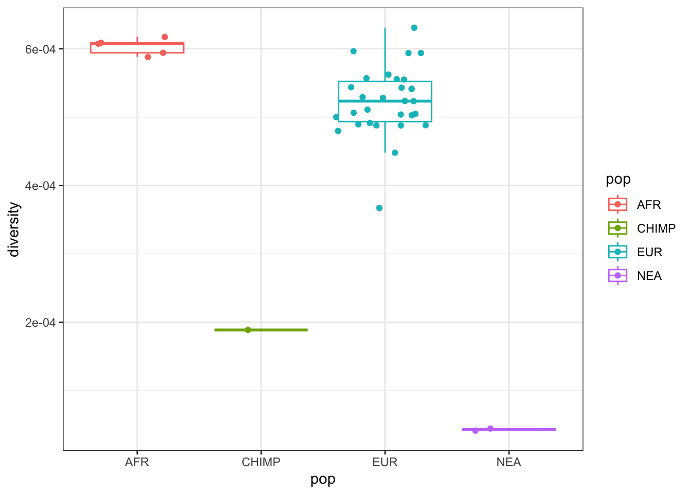
Exercise 2: Computing pairwise divergence
Use the function ts_divergence() to compute genetic divergence between all pairs of populations. Again, do you get results compatible with our demographic model in terms of expectation given the split times between populations as you programmed them for your model?
Hint: Again, you can use the same concept of sample_sets = we discussed in the previous exercise. In this case, the function computes pairwise divergence between each element of the list given as sample_sets = (i.e., for each vector of individual names in that list).
Exercise 3: Outgroup \(f_3\) statistic
**Use the function ts_f3() to compute the outgroup \(f_3\) statistic between pairs of African-European, African-Neanderthal, and European-Neanderthal and a Chimpanzee outgroup. For instance, the first one can be computed as ts_f3(ts, B = "AFR_1", C = "EUR_1", A = "CHIMP_1").
Hint: The \(f_3\) statistic is traditionally expressed as \(f_3(A, B; C)\), where C represents the outgroup. Unfortunately, in tskit the outgroup is named A, with B and C being the pair of samples from which we trace the length of branches towards the outgroup, so the statistic is interpreted as \(f_3(B, C; A).\)
Note: As a reminder, the higher the \(f_3\) value, the more evolutionary time has been shared between samples B and C.
How do the outgroup \(f_3\) results compare to your expectation based on simple population relationships (and to the divergence computation above)?
Do you see any impact of introgression on the \(f_3\) value when a Neanderthal is included in the computation?
Exercise 4: mode = "branch" vs mode = "site"
Repeat the exercise 3 by setting mode = "site" in the ts_f3() function calls (this is actually the default behavior of all slendr tree-sequence based tskit functions). This will switch the tskit computation to using mutation counts along each branch of the tree sequence, rather than using branch length themselves. Why might the branch-based computation be a bit better if what we’re after is investigating the expected values of statistics under some model?
Exercise 5: Outgroup \(f_3\) statistic as a linear combination of \(f_2\) statistics
You might have learned that any complex \(f\)-statistic can be expressed as a linear combination of multiple \(f_2\) statistics (which represent simple branch length separating two lineages). Verify that this is the case by looking up equation (20b) in this amazing paper and computing an \(f_3\) statistic for any arbitrary trio of individuals of your choosing using such linear combination of \(f_2\) statistics.
Hint: Here’s that equation in a schematic form
f3(A, B; C) = f2(A, C) + f2(B, C) - f2(A, B) / 2Exercise 6: Detecting Neanderthal admixture in Europeans
Let’s now pretend its about 2008, we’ve sequenced the first Neanderthal genome, and we are working on a project that will change human evolution research forever. We also have the genomes of a couple of people from Africa and Europe, which we want to use to answer the most burning question of all evolutionary anthropology: “Do some people living today carry Neanderthal ancestry?”
Perhaps you’ve heard earlier about an \(f_4\) statistic (or its equivalent \(D\) statistic) can be used as a test of “treeness”. Simply speaking, for some “quartet” of individuals or population samples (whose names can be giving as characters such as “EUR_1” to the ts_f4() function, as you can see in the help page of ?ts_f4), they can be used as a hypothesis test of whether the history of those samples is compatible with there not having been an introgression.
Compute the \(f_4\) test of Neanderthal introgression in EUR individuals using the slendr function ts_f4().
When you’re computing the \(f_4\), make sure to set mode = "branch" argument of the ts_f4() function.
Note: By default, each slendr / tskit statistic function operates on mutations, and this will switch them to use branch length (as you might know, \(f\)-statistics are mathematically defined using branch lengths in trees and mode = "branch" does exactly that).
Hint: If you haven’t learned this earlier, you want to compute (and compare) the values of these two statistics using the slendr function ts_f4():
\(f_4\)(<some African>, <another African>; <Neanderthal>, <Chimp>)
\(f_4\)(<some African>, <a test European>; <Neanderthal>, <Chimp>),
here <individual> can be the name of any individual recorded in your tree sequence, such as names you saw as name column in the table returned by ts_samples(ts) (i.e. "NEA_1" could be used as a “representative” <Neanderthal> in those equations, similarly for "CHIMP_1" as the fourth sample in the \(f_4\) quarted representing the outgroup).
To simplify things a lot, we can understand the above equations as comparing the counts of so-called BABA and ABBA allele patterns between the quarted of samples specified in the statistics:
\[ f_4(AFR, X; NEA, CHIMP) = \frac{\#BABA - \#ABBA}{\#SNPs} \]
The first \(f_4\) statistic above is not expected to give values “too different” from 0 (even in case of Neanderthal introgression into Europeans) because we don’t expect two African individuals to differ “significantly” in terms of how much alleles they share with a Neanderthal (because their ancestors never met Neanderthals!). The other should — if there was a Neanderthal introgression into Europeans some time in their history — be “significantly negative”.
Is the second of those two statistics “much more negative” than the first, as expected assuming introgression from Neanderthals into Europeans?
Why am I putting “significantly” and “much more negative” in quotes in the previous sentence? What are we missing here for this being a true hypothesis test as you might be accustomed to from computing \(f\)-statistics using a tool such as ADMIXTOOLS? (We will get to this again in a following exercise.)
Exercise 7: Detecting Neanderthal admixture in Europeans v2.0
The fact that we don’t get something equivalent to a p-value in these kinds of simulations is generally not a problem, because we’re often interested in establishing a trend of a statistic under various conditions, and understanding when and how its expected value behaves in a certain way. If statistical noise is a problem, we work around this by computing a statistic on multiple simulation replicates or even increasing the sample sizes.
Note: To see this in practice, you can check out a paper in which I used this approach quite successfully on a related problem.
On top of that, p-value of something like an \(f\)-statistic (whether it’s significantly different from zero) is also strongly affected by quality of the data, sequencing errors, coverage, etc. (which can certainly be examined using simulations!). However, these are aspects of modeling which are quite orthogonal to the problem of investigating the expectations and trends of statistics given some underlying evolutionary model, which is what we’re after in these exercises.
That said, even in perfect simulated data, what exactly does “significantly different from zero compared to some baseline expectation” mean can be blurred by noise with simple single-individual comparisons that we did above. Let’s increase the sample size a bit to see if a statistical pattern expected in \(f_4\) statistic from our Neanderthal introgression model becomes more apparent.
Compute the first \(f_4\) statistic (the baseline expectation between a pair of Africans) and the second \(f_4\) statistic (comparing an African and a European), but this time on all recorded Africans and all recorded Europeans, respectively. Plot the distributions of those two sets of statistics. This should remove lots of the uncertainty and make a statistical trend stand out much more clearly.
Hint: Whenever you need to compute something for many things in sequence, looping is very useful. One way to do compute, say, an \(f_4\) statistic over many individuals is by using this kind of pattern using R’s looping function lapply() (you can get a refresher on looping in the R bootcamp session):
# Loop over vector of individual names (variable x) and apply a given ts_f4()
# expression on each individual (note the ts_f4(..., X = x, ...) in the code)
list_f4 <- lapply(
  c("ind_1", "ind_2", ...),
  function(x) ts_f4(ts, W = "AFR_1", X = x, Y = "NEA_1", Z = "CHIMP_1", mode = "branch")
)

# The above gives us a list of data frames, so we need to bind them all into a
# single table for easier interpretation and visualization
df_f4 <- do.call(rbind, list_f4)
NoteClick to see the solution
This gives us list of vectors of the names of all individuals in each population…
sample_sets <- ts_names(ts, split = "pop")
# ... which we can then access like this
sample_sets$AFR # all Africans
[1] "AFR_1" "AFR_2" "AFR_3" "AFR_4" "AFR_5"sample_sets$EUR # all Europeans [1] "EUR_1" "EUR_2" "EUR_3" "EUR_4" "EUR_5" "EUR_6" "EUR_7" "EUR_8"
[9] "EUR_9" "EUR_10" "EUR_11" "EUR_12" "EUR_13" "EUR_14" "EUR_15" "EUR_16"
[17] "EUR_17" "EUR_18" "EUR_19" "EUR_20" "EUR_21" "EUR_22" "EUR_23" "EUR_24"
[25] "EUR_25" "EUR_26" "EUR_27" "EUR_28" "EUR_29" "EUR_30"Let’s compute the f4 statistic for all Africans…
f4_afr_list <- lapply(
  sample_sets$AFR,
  function(x) ts_f4(ts, W = "AFR_1", X = x, Y = "NEA_1", Z = "CHIMP_1", mode = "branch")
)
# ... and Europeans
f4_eur_list <- lapply(
  sample_sets$EUR,
  function(x) ts_f4(ts, W = "AFR_1", X = x, Y = "NEA_1", Z = "CHIMP_1", mode = "branch")
)
Bind each list of data frames into a single data frame:
f4_afr <- do.call(rbind, f4_afr_list)
f4_eur <- do.call(rbind, f4_eur_list)

# add population columns to each of the two results for easier plotting
f4_afr$pop <- "AFR"
f4_eur$pop <- "EUR"

# bind both tables together
f4_results <- rbind(f4_afr, f4_eur)
Now we can visualize the results:
f4_results %>%
  ggplot(aes(pop, f4, color = pop)) +
  geom_boxplot() +
  geom_jitter() +
  geom_hline(yintercept = 0, linetype = 2) +
  ggtitle("f4(AFR, EUR; NEA, CHIMP)") +
  theme_bw()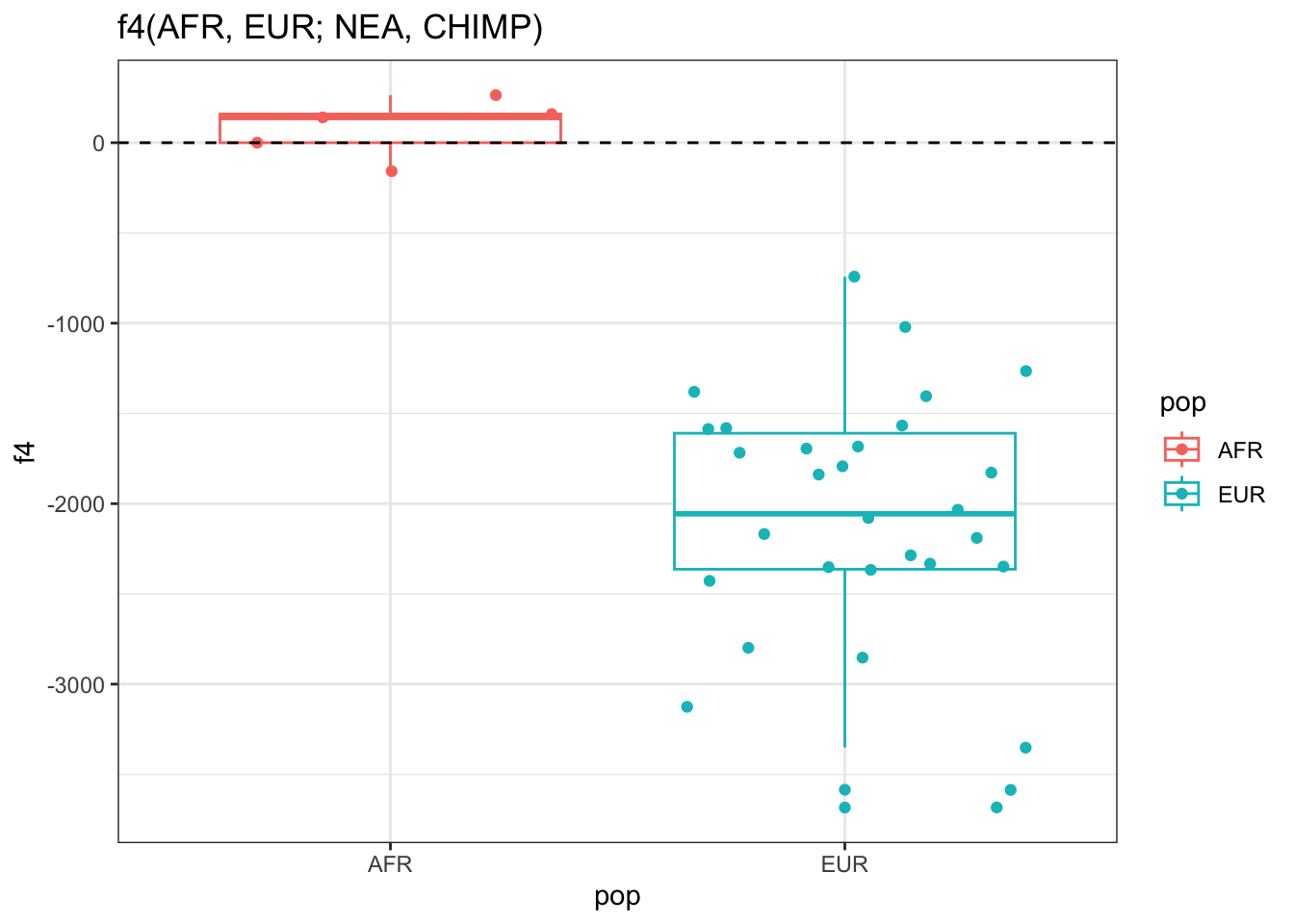
We can see that the \(f_4\) statistic test of Neanderthal introgression in Europeans indeed does give a much more negative distribution of values compared to the baseline expectation which compares two Africans to each other.
Exercise 8: Trajectory of Neanderthal ancestry in Europe over time
There used to be a lot of controversy about the question of whether or not did Neanderthal ancestry proportion in Europeans decline or not over the past 40 thousand years (see Figure 1 in this paper and Figure 2 in this paper).
Your simulated tree sequence contains a time-series of European individuals over time. Use the slendr function ts_f4ratio() to compute (and then plot) the proportion (commonly designated as alpha) of Neanderthal ancestry in Europe over time. Use \(f_4\)-ratio statistic of the following form:
ts_f4ratio(ts, X = <vector of ind. names>, A = "NEA_1", B = "NEA_2", C = "AFR_1", O = "CHIMP_1")
NoteClick to see the solution
# Extract table with names and times of sampled Europeans (ancient and present day)
eur_inds <- ts_samples(ts) %>% filter(pop == "EUR")
eur_inds
# A tibble: 30 × 3
name time pop
<chr> <dbl> <chr>
1 EUR_1 40000 EUR
2 EUR_2 38000 EUR
3 EUR_3 36000 EUR
4 EUR_4 34000 EUR
5 EUR_5 32000 EUR
6 EUR_6 30000 EUR
7 EUR_7 28000 EUR
8 EUR_8 26000 EUR
9 EUR_9 24000 EUR
10 EUR_10 22000 EUR
# ℹ 20 more rows# Compute f4-ration statistic (this will take ~30s) -- note that we can provide
# a vector of names for the X sample set to the `ts_f4ratio()` function
nea_ancestry <- ts_f4ratio(ts, X = eur_inds$name, A = "NEA_1", B = "NEA_2", C = "AFR_1", O = "CHIMP_1")
# Add the age of each sample to the table of proportions
nea_ancestry$time <- eur_inds$time
nea_ancestry# A tibble: 30 × 7
X A B C O alpha time
<chr> <chr> <chr> <chr> <chr> <dbl> <dbl>
1 EUR_1 NEA_1 NEA_2 AFR_1 CHIMP_1 0.0741 40000
2 EUR_2 NEA_1 NEA_2 AFR_1 CHIMP_1 0.0202 38000
3 EUR_3 NEA_1 NEA_2 AFR_1 CHIMP_1 0.0731 36000
4 EUR_4 NEA_1 NEA_2 AFR_1 CHIMP_1 0.0354 34000
5 EUR_5 NEA_1 NEA_2 AFR_1 CHIMP_1 0.0132 32000
6 EUR_6 NEA_1 NEA_2 AFR_1 CHIMP_1 0.0401 30000
7 EUR_7 NEA_1 NEA_2 AFR_1 CHIMP_1 0.0295 28000
8 EUR_8 NEA_1 NEA_2 AFR_1 CHIMP_1 0.0476 26000
9 EUR_9 NEA_1 NEA_2 AFR_1 CHIMP_1 0.0261 24000
10 EUR_10 NEA_1 NEA_2 AFR_1 CHIMP_1 0.0350 22000
# ℹ 20 more rowsnea_ancestry %>%
ggplot(aes(time, alpha)) +
geom_point() +
geom_smooth(method = "lm", linetype = 2, color = "red", linewidth = 0.5) +
xlim(40000, 0) +
coord_cartesian(ylim = c(0, 0.1)) +
labs(x = "time [years ago]", y = "Neanderthal ancestry proportion") +
theme_bw() +
ggtitle("Neanderthal ancestry proportion in Europeans over time")`geom_smooth()` using formula = 'y ~ x'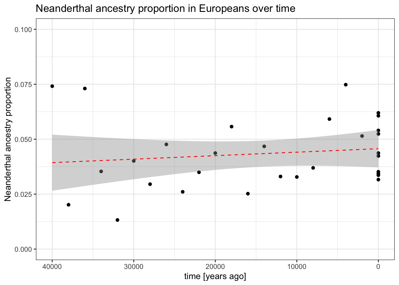
# For good measure, let's test the significance of the decline using a linear model
summary(lm(alpha ~ time, data = nea_ancestry))
Call:
lm(formula = alpha ~ time, data = nea_ancestry)

Residuals:
      Min        1Q    Median        3Q       Max
-0.027358 -0.011309 -0.002650  0.007912  0.034803

Coefficients:
              Estimate Std. Error t value Pr(>|t|)
(Intercept)  4.569e-02  4.153e-03  11.001 1.13e-11 ***
time        -1.588e-07  2.123e-07  -0.748    0.461
---
Signif. codes:  0 '***' 0.001 '**' 0.01 '*' 0.05 '.' 0.1 ' ' 1

Residual standard error: 0.01589 on 28 degrees of freedom
Multiple R-squared:  0.0196,    Adjusted R-squared:  -0.01541
F-statistic: 0.5598 on 1 and 28 DF,  p-value: 0.4606
Exercise 9 (hard challenge): How many unique f4 quartets are there?
If you’ve used \(f\)-statistics before, you’ve probably learned about various symmetries in \(f_4\) (but also other \(f\)-statistics) depending on the arrangement of the “quartet”. As a trivial example, an \(f_3(A; B, C)\) and \(f_3(A; C, B)\) will give you exactly the same value, and the same thing applies even to more complex \(f\)-statistics like \(f_4\).
Use simulations to compute how many unique \(f_4\) values involving a single quartet are there.
Hint: Draw some trees to figure out why could that be true. Also, when computing ts_f4(), set mode = "branch" to avoid the effect of statistical noise due to mutations.