# here
# is
# some
123
# R
"code"R bootcamp
In this first chapter, you will be exploring the fundamental, more technical aspects of the R programming language. We will focus on topics which are normally taken for granted and never explained in basic data science courses, which generally immediately jump to data manipulation and plotting.
I strongly believe that getting familiar with the fundamentals of R as a complete programming language from a “lower-level” perspective, although it might seem a little overwhelming at the beginning, will pay dividends over and over your scientific career.
The alternative is relying on magical black box thinking, which might work when everything works smoothly… except things rarely work smoothly in anything related to computing. Bugs appear, programs crash, incorrect results are produced—only by understanding the fundamentals can you troubleshoot problems.
We call this chapter a “bootcamp” on purpose – we only have a limited amount of time to go through all of these topics, and we have to rush things through a bit. After all, the primary reason for the existence of this workshop is to make you competent researchers in computational population genomics, so the emphasis will still be on practical applications and solving concrete data science issues.
Still, when we get to data science work in the following chapters, you will see that many things which otherwise remain quite obscure and magical boil down to a set of very simple principles introduced here. The purpose of this chapter is to show you these fundamentals.
This knowledge will make you much more confident in the results of your work, and much easier to debug issues and problems in your own projects, but also track down problems in other people’s code. The later happens much more often than you might think!
Getting help
Before we even get started, there’s one thing you should remember: R (and R packages) have an absolutely stellar documentation and help system. What’s more, this documentation is standardized, has always the same format, and is accessible in the same way. The primary way of interacting with it from inside R (and RStudio) is the ? operator. For instance, to get help about the hist() function (histograms), you can type ?hist in the R console. This documentation has a consistent format and appears in the “Help” pane in your RStudio window.
There are a couple of things to look for:
On the top of the documentation page, you will always see a brief description of the arguments of each function. This is what you’ll be looking for most of the time (“How do I do specify this or that? How do I modify the behavior of the function?”).
On the bottom of the page are examples. These are small bits of code which often explain the behavior of some functionality in a very helpful way.
Whenever you’re lost or can’t remember some detail about some piece of R functionality, looking up ? documentation is always very helpful.
As a practice and to build a habit, whenever we introduce a new function like new_function() in this course, use ?new_function to open its documentation and skim through it. I do this many times a day to refresh my memory on how something works.
Exercise 0: Creating an R Script and general workflow
Let’s start easy. Open RStudio, create a new R script (File -> New file -> R Script), save it somewhere on your computer as r-bootcamp.R (File -> Save, doesn’t really matter where you save it).
Every time you encounter a new bit of code, looking like this (i.e., text shown in a grey box like this):
please copy it into your script. You can then put your cursor on the first line of that code, and hit CTRL + Enter (on Windows/Linux) or CMD + Enter (on macOS) to execute it, which will step over to the next executable line. (Generally up to the next following # comment block prefixed with '#'). Alternatively, you can also type it out to the R Console directly, and evaluate it by hitting Enter.
It will sound very annoying, but try to limit copy-pasting code only to very long commands. Typing things out by hand forces you to think about every line of code and that is very important! At least at the beginning.
Exercise 1: Basic data types and variables
Every time you create a value in R, an object is created in computer memory. For instance, when you type this and execute this command in the R console by pressing Enter, R creates a bit of text in memory:
"this is a bit of text"You can use the assignment operator in R <- to store an object in a variable, here a variable called text_var:
text_var <- "this is a bit of text"Except saying that this “stores and object in a variable” is not correct, even though we always use this phrase. Instead, the <- operator actually stores a reference to a bit of computer memory where that value is located. This means that even after you run this command next, "this is a bit of text" is still sitting in memory, even though it appears to have been overwritten by the number 42 (we just don’t have access to that text anymore):
text_var <- "this is a bit of text"
text_var <- 42
Similarly, when you run this bit of code, you don’t create a duplicate of that text value, the second variable refers to the same bit of computer memory:
text_var1 <- "some new text value"
text_var2 <- text_var1
To summarize: values (lines of text, numbers, data frames, matrices, lists, etc.) don’t have “names”. They exist “anonymously” in computer memory. Variables are nothing but “labels” for those values.
It might be very strange to start with something this technical (and almost philosophical!), but it is very much worth keeping this in mind, especially in more complex and huge data sets which we’ll get to later in our workshop.
We will continue saying things like “variable abc contains this or that value” (instead of “contains reference to that value in memory”) because of convenience, but this is just an oversimplification.
Write the following variable definitions in your R script and then evaluate this code in your R console by CTRL / CMD + Enter. (Note that hitting this shortcut will move the cursor to the next line, allowing you to step by step evaluate longer bits of code.)
w1 <- 3.14
x1 <- 42
y1 <- "hello"
z1 <- TRUE
When you type the variable names in your R console, you’ll get them printed back, of course:
w1[1] 3.14x1[1] 42y1[1] "hello"z1[1] TRUEProgramming involves assigning values (or generally some objects in computer memory in general) to variables. In our code, variables change values, so we often need to check what is a type of some variable—are we working with a number, or some text, etc.? typeof() is one of the functions that are useful for this.
What are the data “types” you get when you apply function typeof() on each of these variables, i.e. when you type and evaluate a command like typeof(w1)? Compare the result to the values you saved in those variables—what do you get from typeof() on each of them?
You can test whether or not a specific variable is of a specific type using functions such as is.numeric(), is.integer(), is.character(), is.logical(). See what results you get when you apply these functions on these four variables w1, x1, y1, z1. Pay close attention to the difference (or lack thereof?) between applying is.numeric() and is.integer() on variables containing “values which look like numbers” (42, 3.14, etc.).
Note: This might seem incredibly boring and useless but trust me. In your real data, such as in data frames (discussed below), you will encounter variables with thousands of rows, sometimes millions. Being able to make sure that the values you get in your data-frame columns are of the expected type is something you will be doing very very often, especially when troubleshooting! So this is a good habit to get into.
To summarize (and oversimplify a little bit) R allows variables to have several types of data, most importantly:
- integers (such as
42) - numerics (such as
42.13) - characters (such as
"text value") - logicals (
TRUEorFALSE)
We will also encounter two types of “non-values”. We will not be discussing them in detail here, but they will be relevant later. For the time being, just remember that there are also:
- missing values represented by
NA—you will see this very often in data! - undefined values represented by
NULL
What do you think is the practical difference between NULL and NA? In other words, when you encounter one or the other in the data, how would you interpret this?
Exercise 2: Vectors
Vectors are, roughly speaking, collections of values. We create a vector by calling the c() function (the “c” stands for “concatenate”, or “joining together”).
Create the following variables containing these vectors. Then inspect their data types by calling the typeof() function on them again, just like you did for “single-value variables” above. Again, copy-paste this into your script and evaluate using CTRL / CMD + Enter or paste it directly into your R Console and hit Enter:
w2 <- c(1.0, 2.72, 3.14)
x2 <- c(1, 13, 42)
y2 <- c("hello", "folks", "!")
z2 <- c(TRUE, FALSE)We can use the function is.vector() to test that a given object really is a vector. Try this on your vector variables.
What happens when you call is.vector() on the variables x1, y1, etc. from the previous Exercise (i.e., those which contain single values)?
Do elements of vectors need to be homogeneous (i.e., of the same data type)? Try creating a vector with values 1, "42", and "hello" using the c() function again, maybe save it into the variable mixed_vector. Can you do it? What happens when you try (and evaluate this variable in the R console)? Inspect the result in the R console (take a close look at how the result is presented in text and the quotes that you will see), or use the typeof() function again.
You can see that if vectors are not created with values of the same type, they are converted by a cascade of so-called “coercions”. A vector defined with a mixture of different values (i.e., the four “atomic types” we discussed in Exercise 1, doubles, integers, characters, and logicals) will be coreced to be only one of those types, given certain rules.
Do a little detective work and try to figure out some of these coercion rules. Make a couple of vectors with mixed values of different types using the function c(), and observe what type of vector you get in return.
Hint: Try creating a vector which has integers and strings, integers and decimal numbers, integers and logicals, decimals and logicals, decimals and strings, and logicals and strings. Observe the format of the result that you get, and build your intuition on the rules of coercions by calling typeof() on each vector object to verify this intuition.
Out of all these data type explorations, this Exercise is probably the most crucial for any kind of data science work. Why do you think I say this? Think about what can happen when someone does incorrect manual data entry in Excel.
Although creating vectors manually c("using", "an", "approach", "like", "this") is often helpful, particularly when testing bits of code and experimenting in the R console, it is impossible to create dozens or more values like this by hand.
You can create vector of consecutive values using several useful approaches. Try and experiment these options:
Create a sequence of values from
itojwith a shortcuti:j. Create a vector of numbers from 7 to 23 like this.Do the same using the function
seq(). Read?seqto find out what parameters you should specify (and how) to get the same result as thei:jshortcut above to get vector 7 to 23.Modify the arguments given to
seq()so that you create a vector of numbers from 20 to 1.Use the
by =argument ofseq()to create a vector of only odd values starting from 1.
seq() is one of the most useful utility functions in R, so keep it in mind!
Another very useful built-in helper function (especially when we get to the iteration Exercise below) is seq_along(). What does it give you when you run it on this vector, for instance?
v <- c(1, "42", "hello", 3.1416)Exercise 3: Lists
Lists (created with the list() function, equivalent to the c() function for vectors) are a little similar to vectors but very different in a couple of important respects. Remember how we tested what happens when we put different types of values in a vector (reminder: vectors must be “homogeneous” in terms of the data types of their elements!)?
What happens when you create lists with different types of values using the code in the following chunk? Use typeof() on the resulting list variables and compare your results to those you got on “mixed value” vectors above.
w3 <- list(1.0, "2.72", 3.14)
x3 <- list(1, 13, 42, "billion")
y3 <- list("hello", "folks", "!", 123, "wow a number follows again", 42)
z3 <- list(TRUE, FALSE, 13, "string")Calling typeof() on the list in the R console will (disappointingly) not tell us much about the data types of each individual element. Why is that? Think about the mixed elements possible in a list.
Try also a different function called for str() (“str” standing for “structure”) and apply it on one of those lists in your R console. Is typeof() or str() more useful to inspect what kind of data is stored in a list (str will be very useful when we get to data frames for — spoiler alert! — exactly this reason). Why?
Apply is.vector() and is.list() on one of the lists above (like w3 perhaps). What result do you get? Why do you get that result? Then run both functions on one of the vectors you created above (like w2). What does this mean?
Not only can lists contain arbitrary values of mixed types (atomic data types from Exercise 1 of this exercise), they can also contain “non-atomic” data as well, such as other lists! In fact, you can, in principle, create lists of lists of lists of… lists!
Try creating a list() which, in addition to a couple of normal values (numbers, strings, doesn’t matter) also contains one or two other lists (we call these lists “nested lists” for this reason, or also “recursive lists”). Don’t think about this too much, just create something arbitrary “nested lists” to get a bit of practice. Save this in a variable called weird_list and type it back in your R console, just to see how R presents such data back to you. In the next Exercise, we will learn how to explore this type of data better.
Note: If you are confused (or even annoyed) why we are even doing this, in the later discussion of data frames and spatial data structures, it will become much clearer why putting lists into other lists allows a whole another level of data science work. Please bear with me for now! This is just laying the groundwork for some very cool things later down the line… and, additionally, it’s intended to bend your mind a little bit and get comfortable with how complex data can be represented in computer memory.
Exercise 4: Logical/boolean expressions and conditionals
This exercise is probably the most important thing you can learn to do complex data science work on data frames or matrices. It’s not necessary to remember all of this, just keep in mind we did these exercise so that you can refer to this information on the following days!
Let’s recap some basic Boolean algebra in logic. The following basic rules apply (take a look at the truth table for a bit of a high school refresher) for the “and”, “or”, and “negation” operations:
- The AND operator (represented by
&in R, or often∧in math):
Both conditions must be TRUE for the expression to be TRUE.
TRUE&TRUE==TRUETRUE&FALSE==FALSEFALSE&TRUE==FALSEFALSE&FALSE==FALSE
- The OR operator (represented by
|in R, or often∨in math):
At least one condition must be TRUE for the expression to be TRUE.
TRUE|TRUE==TRUETRUE|FALSE==TRUEFALSE|TRUE==TRUEFALSE|FALSE==FALSE
- The NOT operator (represented by
!in R, or often¬in math):
The negation operator turns a logical value to its opposite.
!TRUE==FALSE!FALSE==TRUE
- Comparison operators
==(“equal to”),!=(“not equal to”),<or>(“lesser / greater than”), and<=or>=(“lesser / greater or equal than”):
Comparing two things with either of these results in TRUE or FALSE result.
Note: There are other operations and more complex rules, but we will be using these four exclusively (plus, the more complex rules can be derived using these basic operations anyway).
Let’s practice working with logical conditions on some toy problems.
Create two logical vectors with three elements each using the c() function (pick random TRUE and FALSE values for each of them, it doesn’t matter at all), and store them in variables named A and B. What happens when you run A & B, A | B, and !A or !B in your R console? How do these logical operators work when you have multiple values, i.e. vectors?
For extra challenge, try to figure out the results of A & B, A | B, and !A in your head before you run the code in your R console!
Hint: Remember that a “single value” in R is a vector like any other (specifically vector of length one).
What happens when you apply base R functions all() and any() on your A and B (or !A and !B) vectors?
Note: Remember the existence of all() and any() because they are very useful in daily data science work!
If the above all feels too technical and mathematical, you’re kind of right. That said, when you do data science, you will be using these logical expressions literally every single day. Why? Let’s return from abstract programming concepts back to reality for a second.
Think about a table which has a column with some values, like sequencing coverage. Every time you filter for samples with, for instance, coverage > 10, you’re performing exactly this kind of logical operation. You essentially ask, for each sample (each value in the column), which samples have coverage > 10 (giving you TRUE) and which have less than 10 (giving you FALSE).
Filtering data is about applying logical operations on vectors of TRUE and FALSE values (which boils down to “logical indexing” introduced below), even though those logical values rarely feature as data in the tables we generally work with. Keep this in mind!
Consider the following vectors of coverages and origins of some set of example aDNA individuals (let’s imagine these are columns in a table you got from a bioinformatics lab) and copy them into your R script:
coverage <- c(15.09, 48.85, 36.5, 47.5, 16.65, 0.79, 16.9, 46.09, 12.76, 11.51)
origin <- c("mod", "mod", "mod", "anc", "mod", "anc", "mod", "mod", "mod", "mod")
Then create a variable is_high which will contain a TRUE / FALSE vector indicating whether a given coverage value is higher than 10. Then create a variable is_ancient which will contain another logical vector indicating whether a given sample is "anc" (i.e., “ancient”).
Hint: Remember that evaluating coverage > 10 gives you a logical vector and that you can store that vector in a variable.
Use the AND operator & to test if there is any high coverage sample (is_high) which is also ancient (is_ancient).
Hint: Apply the any() function to a logical expression you get by comparing both variables using the & operation.
Now let’s say that you have a third vector in this hypothetical table, indicating whether or not is a given sample from Estonia:
estonian <- c(FALSE, TRUE, FALSE, TRUE, FALSE, TRUE, FALSE, TRUE, FALSE,
FALSE)
Write now a more complex conditional expression, which will test if a given individual has (again) coverage higher than 10 and is “ancient” OR whether it’s Estonian (and so it’s coverage or “mod” state doesn’t matter).
This was just a simple example of how you can use logical expressions to do filtering based on values of (potentially many) variables, all at once, in a so-called “vectorized” way (i.e., testing on many different values at once, getting a vector of TRUE / FALSE values as a result).
You’ll have much more opportunity to practice this in our sessions on tidyverse, but let’s continue with other fundamentals first, which will make your understanding of basic data manipulation principles even more solid.
R has also equivalent operators && and ||. What do they do and how are they different from the & and | you already worked with? Pick some exercises from above and experiment with both versions of logical AND and OR operators to figure out what they do and how are they different.
Exercise 5: Indexing into vectors and lists
Vectors and lists are sequential collections of values.
To extract a specific values(s) of a vector or a list (or to assign some value at its given position(s)), we use a so-called “indexing” operation (often also called “subsetting” operation for reasons that will become clear soon). Generally speaking, we can do indexing in three ways:
numerical-based indexing (by specifying a set of integer numbers, each representing a position in the vector/list we want to extract),
logical-based indexing (by specifying a vector of
TRUE/FALSEvalues of the same length as the vector/list we’re indexing into, each representing whether or not –TRUEorFALSE– should a position be included in the indexing result)name-based indexing (by specifying names of elements to index)
Let’s now practice those for vectors and lists separately. Later, when we introduce data frames, we will return to the topic of indexing again.
Vectors
1. Numerical-based indexing
To extract an i-th element of a vector xyz, we can use the [] operator like this: xyz[i]. For instance, we can take the 13-th element of this vector as xyz[13].
Familiarize yourselves with the [] operator by taking out a specific value from this vector, let’s say its 5th element.
v <- c("hi", "folks", "what's", "up", "folks")Like many operations in R, the [] operator is “vectorized”, meaning that it can actually accept multiple values given as a vector themselves (i.e, something like v[c(1, 3, 4)] will extract the first, third, and fourth element of the vector v.
Extract the first and fifth element of the vector v. What happens if you try to extract a tenth element from v?
2. Logical-based indexing
Rather than giving the [] operator a specific set of integer numbers, we can provide a vector of TRUE / FALSE values which specify which element of the input vector do we want to “extract”. Note that this TRUE / FALSE indexing vector must have the same length as our original vector!
Create variable containing a vector of five TRUE or FALSE values (i.e., with something like index <- c(TRUE, FALSE, ...), the exact combination of logical values doesn’t matter), and use that index variable in a v[index] indexing operation on the v vector you created above.
Note: As always, don’t forget that you can experiment in your R Console, write bits of “throwaway” commands just to test things out. You don’t have to “know” how to program something immediately in your head—I never do, at least. I always experiment in the R Console to build up understanding of some problem on some small example.
Usually we never want to create this “indexing vector” manually (imagine doing this for a vector of million values – impossible!). Instead, we create this indexing vector “programmatically”, based on a certain expression which produces this TRUE / FALSE indexing vector as a result (or multiple such expressions combined with &, | and ! operations), like this:
# v is our vector of values
v
[1] "hi" "folks" "what's" "up" "folks" # this is how we get the indexing vector to get only positions matching
# some condition
index <- v == "up"This checks which values of v are equal to “three”, creating a logical TRUE / FALSE vector in the process, storing it in the variable index:
index[1] FALSE FALSE FALSE TRUE FALSEUse the same principle to extract the elements of the vector v matching the value “folks”.
Note: As always, don’t forget that you can experiment in your R Console, write bits of “throwaway” commands just to test things out.
A nice trick is that summing a logical vector using sum() gives you the number of TRUE matches:
index[1] FALSE TRUE FALSE FALSE TRUEsum(index)[1] 2This is actually why we do this indexing operation on vectors in the first place, most of the time — when we want to count how many data points match a certain criterion.
There’s another very useful operator is %in%. It tests which elements of one vector are among the elements of another vector. This is another extremely useful operation which you will be doing all the time when doing data analysis. It’s good for you to get familiar with it.
For instance, if we take this vector again:
v <- c("hi", "folks", "what's", "up", "folks", "I", "hope", "you",
       "aren't", "(too)", "bored")
You can then ask, for instance, “which elements of v are among a set of given values?” by writing this command:
v %in% c("folks", "up", "bored") [1] FALSE TRUE FALSE TRUE TRUE FALSE FALSE FALSE FALSE FALSE TRUEWith our example vector v, it’s very easy to glance this with our eyes, of course. But when working with real world data, we often operate on tables with thousands or even millions of columns.
Try the above example of using the %in% operator in your R Console to get familiar with.
Let’s imagine we don’t need to test whether a given vector is a part of a set of pre-defined values, but we want to ask the opposite question: “are any of my values of interest in my data”? Let’s say your values of interest are values <- c("hope", "(too)", "blah blah") and your whole data is again v. How would you use the %in% operator to get a TRUE / FALSE vector for each of your values?
Lists
We went through the possibilities of indexing into vectors.
This section will be a repetition on the previous exercises about vectors. Don’t forget — lists are just vectors, except that they can contain values of heterogeneous types (numbers, characters, anything). As a result, everything that applies to vectors above applies also here.
But practice makes perfect, so let’s go through a couple of examples anyway. Run this code to create the following list variable:
l <- list("hello", "folks", "!", 123, "wow a number follows again", 42)
l
[[1]]
[1] "hello"
[[2]]
[1] "folks"
[[3]]
[1] "!"
[[4]]
[1] 123
[[5]]
[1] "wow a number follows again"
[[6]]
[1] 421. Numerical-based indexing
The same applies to numerical-based indexing as what we’ve shown for vectors.
Extract the second and fourth elements from l.
2. Logical-based indexing
Similarly, you can do the same with TRUE / FALSE indexing vectors for lists as what we did with normal vectors. Rather than go through the variation of the same exercises, let’s introduce another very useful pattern related to logical-based indexing and that’s removing invalid elements.
Consider this list (run this code in your R Console again):
xyz <- list("hello", "folks", "!", NA, "wow another NAs are coming", NA, NA, "42")

xyz
[[1]]
[1] "hello"
[[2]]
[1] "folks"
[[3]]
[1] "!"
[[4]]
[1] NA
[[5]]
[1] "wow another NAs are coming"
[[6]]
[1] NA
[[7]]
[1] NA
[[8]]
[1] "42"Notice the NA values. One operation we have to do very often (particularly in data frames, whose columns are vectors as we will see below!) is to remove those invalid elements, using the function is.na().
This function returns a TRUE / FALSE vector which, as you now already know, can be used for logical-based indexing!
is.na(xyz)[1] FALSE FALSE FALSE TRUE FALSE TRUE TRUE FALSEAs you’ve seen in the section on logical expressions, a very useful trick in programming is negation (using the ! operator), which flips the TRUE / FALSE states. In other words, prefixing with ! returns a vector saying which elements of the input vector are not NA:
!is.na(xyz)[1] TRUE TRUE TRUE FALSE TRUE FALSE FALSE TRUEUse is.na(xyz) and the negation operator ! to remove the NA elements of the list from the variable xyz!
[] vs [[ ]] operators
Let’s move to a topic which can be quite puzzling for a lot of people. There’s another operator useful for lists, and that’s [[ ]] (not [ ]!). Extract the third element of the list l using l[4] and l[[4]]]. What’s the difference between the results? If you’re unsure, use the already familiar typeof() function on l[3] and l[[3]] to help you.
NoteClick to see the solution
Strange, isn’t it? The [ ] operator seems to return a list, even though we expect the result 123?
l[4][[1]]
[1] 123typeof(l[4])[1] "list"On the other hand, l[[4]] gives us just a number!
l[[4]][1] 123typeof(l[[4]])[1] "double"I simply cannot not link to this brilliant figure, which explains this result in a very fun way:
The left picture shows our list l, the middle picture shows l[4], the right picture shows l[[4]]. Spend some time experimenting with the behavior of [ ] and [[ ]] on our list l! This will come in handy many times in your R carreer!
Named indexing for vectors and lists
Here’s a neat thing we can do with vectors and lists. They don’t have to contain just values themselves (which can be then extracted using integer or logical indices as we’ve done above), but those values can be assigned names too.
Consider this vector and list (create them in your R session console):
v <- c(1, 2, 3, 4, 5)
v
[1] 1 2 3 4 5l <- list(1, 2, 3, 4, 5)
l[[1]]
[1] 1
[[2]]
[1] 2
[[3]]
[1] 3
[[4]]
[1] 4
[[5]]
[1] 5As a recap, we can index into them in the usual manner like this:
# extract the first, third, and fifth element
v[c(1, 3, 5)]
## [1] 1 3 5
l[c(1, 3)]
## [[1]]
## [1] 1
##
## [[2]]
## [1] 3
But we can also name the values like this (note that the names appear in the print out you get from R in the console):
v <- c(first = 1, second = 2, third = 3, fourth = 4, fifth = 5)
v
first second third fourth fifth
1 2 3 4 5 l <- list(first = 1, second = 2, third = 3, fourth = 4, fifth = 5)
l$first
[1] 1
$second
[1] 2
$third
[1] 3
$fourth
[1] 4
$fifth
[1] 5When you have a named data structure like this, you can index into it using those names and not just integer numbers, which can be very convenient. Imagine having data described not by indices but actually readable names (such as names of people, or excavation sites!). Try this:
l[["third"]][1] 3l[c("second", "fifth")]$second
[1] 2
$fifth
[1] 5Note: This is exactly what data frames are, under the hood (named lists!), as we’ll see in the next section.
For named list, an alternative, more convenient means to select an element by its name is a $ operator. I’m mentioning it here in the section on lists, but it is most commonly used with data frames:
# note the lack of "double quotes"!
l$third
[1] 3Negative indexing
A final topic on indexing (I think you are quite convinced now how crucial role does indexing play in data science in R)—negative indices.
Consider this vector again:
v <- c("hi", "folks", "what's", "up", "folks")What happens when you index into v using the [] operator but give it a negative number between 1 and 5?
In this context, a very useful function is length(), which gives the length of a given vector (or a list — remember, lists are vectors!). Use length() to remove the last element of v using the idea of negative indexing.
How would you remove both the first and last element of a vector or a list (assuming you don’t know the length beforehand, i.e., you can’t put a fixed number as the index of the last element)?
Hint: Remember that you can use a vector created using the c() function inside the [ ] indexing operator.
Exercise 6: Data frames
Every scientists works with tables of data, in one way or another. R provides first class support for working with tables, which are formally called “data frames”. We will be spending most of our time of this workshop learning to manipulate, filter, modify, and plot data frames, usually using example data too big to look at all at once.
Therefore, for simplicity, and just to get started and to explain the basic fundamentals, let’s begin with something trivially easy, like this little data frame here (evaluate this in your R Console):
df <- data.frame(
  v = c("one", "two", "three", "four", "five"),
  w = c(1.0, 2.72, 3.14, 1000.1, 1e6),
  x = c(1, 13, 42, NA, NA),
  y = c("folks", "hello", "from", "data frame", "!"),
  z = c(TRUE, FALSE, FALSE, TRUE, TRUE)
)

df
v w x y z
1 one 1.00 1 folks TRUE
2 two 2.72 13 hello FALSE
3 three 3.14 42 from FALSE
4 four 1000.10 NA data frame TRUE
5 five 1000000.00 NA ! TRUEFirst, here’s the first killer bit of information: data frames are normal lists of vectors!
is.list(df)[1] TRUEHow is this even possible? And why is this even the case? Explaining this in full would be too much detail, even for a course which tries to go beyond “R only as a plotting tool” as I promised you in the introduction. Still, for now let’s say that R objects can store so called “attributes” (normally hidden), which — in the case of data frame objects — makes them behave as “something more than just a list”. These hidden attributes are called “classes”. A list with this class attribute called “data frame” then behaves like a data frame, i.e. a table.
You can poke into these internals but “unclassing” an object, which removes that hidden “class” attribute. Call unclass(df) in your R console and observe what result you get..
Note: Honest admission on my part — you will never need this unclass() stuff in practice, ever. I’m really showing you to demonstrate what “data frame” actually is on a lower-level of R programming. If you’re confused, don’t worry. The fact that data frames are lists matters infinitely more than knowing exactly how is that accomplished inside R.
Bonus exercise
Feel free to skip unless you are a more advanced R user and are interested in the very technical internal peculiarities of R data frames and their relationships to lists.
So, remember how we talked about “named lists” in the previous section? Yes, data frames really are just normal named lists with extra bit of behavior added to them (namely the fact that these lists are printed in a nice, readable, tabular form).
Selecting columns
Quite often we need to extract values of an entire column of a data frame. In the Exercise about indexing, you have learned about the [] operator (for vectors and lists), and also about the $ and [[]] operator (for lists). Now that you’ve learned that data frames are (on a lower level) just lists, what does it mean for wanting to extract a column from a data frame?
Try to use the three indexing options to extract the column named "z" from your data frame df. How do the results differ depending on the indexing method chosen? Is the indexing (and its result) different to indexing a plain list? Create a variable with the list with the same vectors as are in the columns of the data frame df to answer the last question.
The tidyverse approach
In the chapter on tidyverse, we will learn much more powerful and easier tools to do these types of data-frame operations, particularly the select() function which selects specific columns of a table. That said, even when you use tidyverse exclusively, you will still encounter code in the wild which uses this base R way of doing things. Additionally, for certain trivial actions, doing “the base R thing” is just quicker to types. This is why knowing the basics of $, [ ], and [[ ]] will always be useful. I use them every day.
Selecting rows (“filtering”)
Of course, we often need to refer not just to specific columns of data frames (which we do with the $, [ ], and [[ ]] operators), but also to given rows. Let’s consider our data frame again:
df v w x y z
1 one 1.00 1 folks TRUE
2 two 2.72 13 hello FALSE
3 three 3.14 42 from FALSE
4 four 1000.10 NA data frame TRUE
5 five 1000000.00 NA ! TRUEIn the section on indexing into vectors and lists above, we learned primarily about two means of indexing into vectors. Let’s revisit them in the context of data frames:
1. Integer-based indexing
What happens when you use the [1:3] index into the df data frame, just as you would do by extracting the first three elements of a vector?
When indexing into a data frame, you need to distinguish the dimension along which you’re indexing: either a row, or a column dimension. Just like in referring to a cell coordinate in Excel, for example.
The way you do this for data frames in R is to separate the dimensions into which you’re indexing with a comma in this way: df[row indices, column names].
Extract the first three rows (1:3) of the data frame df.
Then select a subset of the df data frame to only show the first and fourth row and columns "x" and "z".
2. Logical-based indexing
Similarly to indexing into vectors, you can also specify which rows should be extracted “at once”, using a single logical vector (you can also do this for columns but I honestly don’t remember the last time I had to do this).
The most frequent use for this is to select all rows of a data frame for which a given column (or multiple columns) carry a certain value.
Select only those rows of df for which the column “y” has a value “hello”:
Hint: You can get the required TRUE / FALSE indexing vector with df$y == "hello". Again, if you’re confused, first evaluate this expression in your R console, then try to use it to filter the rows of the data frame df to get your answer.
Now, instead of filtering rows where column y matches “hello”, filter for rows of the df data frame where w column is less than 1000.
Hint: Same idea as above — first get the TRUE / FALSE vector indicating which rows of the data frame (alternatively speaking, which elements of the column/vector) pass the filtering criterion, then use that vector as a row index into the data frame.
Remember how we used to filter out elements of a vector using the !is.na(...) operation? You can see that df contains some NA values in the x column. Use the fact that you can filter rows of a data frame using logical-based vectors (as demonstrated above) to filter out rows of df at which the x column contains NA values.
Hint: You can get indices of the rows of df we you want to retain with !is.na(df$x).
Creating, modifying, and deleting columns
The $ and [ ] operators can be used to create, modify, and delete columns.
Creating a column
The general pattern to create a new column is this:
df$NAME_OF_THE_NEW_COLUMN <- VECTOR_OF_VALUES_TO_ASSIGN_AS_THE_NEW_COLUMNor this:
df["NAME_OF_THE_NEW_COLUMN"] <- VECTOR_OF_VALUES_TO_ASSIGN_AS_THE_NEW_COLUMNFor instance, the paste() function in R can be used to combine a pair of values into one. Try running paste(df$v, df$y) to see what the result of this operation is.
Create a new column of df called "new_col" and assign to it the result of paste(df$v, df$y). Try to guess what will be this column’s values before you write and evaluate the code for your answer!
Modifying a column
The above pattern doesn’t only apply to creating new columns. You can also update and change values of existing columns using the same technique!
Our data frame df has the following values in the column z:
df$z[1] TRUE FALSE FALSE TRUE TRUEInvert the logical values of this column using the ! negation operator. In other words, the values of the modified column should be the result of !df$z.
Removing a column
When we want to remove a column from a data frame (for instance, we only used it to store some temporary result in a script), we actually do the same thing, except we assign to it the value NULL.
Remove the column new_col using this technique.
“Improper” column names
Most column names you will be using in your own script will (well, should!) follow the same rules as apply for variable names – they can’t start with a number, have to compose of alphanumeric characters, and can’t contain any other characters except for underscores (and occasionally dots). To quote from the venerable R language reference:
Identifiers consist of a sequence of letters, digits, the period (‘.’) and the underscore. They must not start with a digit or an underscore, or with a period followed by a digit.
For instance, these are examples of proper identifiers which can serve as variable names, column names and (later) function names:
variable1a_longer_var_42anotherVariableName
Unfortunately, when you encounter data in the wild, especially in tables you get from other people or download as supplementary information from the internet, they are rarely this perfect. Here’s a little example of such data frame (evaluate this code to have it in your R session as weird_df):
weird_df <- data.frame(
  `v with spaces` = c("one", "two", "three", "four", "five"),
  w = c(1.0, 2.72, 3.14, 1000.1, 1e6),
  `y with % sign` = c("folks", "hello", "from", "data frame", "!")
)
names(weird_df) <- c("v with spaces", "w", "y with % sign")
weird_df v with spaces w y with % sign
1 one 1.00 folks
2 two 2.72 hello
3 three 3.14 from
4 four 1000.10 data frame
5 five 1000000.00 !If you look closely, you see that some columns have spaces " " and also strange characters % which are not allowed. Which of the $, [ ] and [[ ]] operators can you use to extract columns named "v with spaces" and "y with % sign" columns as vectors?
The tidyverse approach
Similarly to previous section on column selection, there’s a much more convenient and faster-to-type way of doing filtering, using the tidyverse function filter(). Still, as with the column selection, sometimes doing the quick and easy thing is just more convenient. The minimum on filtering rows of data frames introduced in this section will be enough for you, even in the long run!
Exercise 7: Inspecting column types
Let’s go back to our example data frame. Create it in your R session as the variable df1 by running this code:
df1 <- data.frame(
  w = c(1.0, 2.72, 3.14),
  x = c(1, 13, 42),
  y = c("hello", "folks", "!"),
  z = c(TRUE, FALSE, FALSE)
)

df1
w x y z
1 1.00 1 hello TRUE
2 2.72 13 folks FALSE
3 3.14 42 ! FALSEUse the function str() and by calling str(df1), inspect the types of columns in the table.
Sometimes (usually when we read data from disk, like from another software), a data point sneaks in which makes a column apparently non numeric. Consider this new table called df2 (evaluate this in your R session too):
df2 <- data.frame(
  w = c(1.0, 2.72, 3.14),
  x = c(1, "13", 42.13),
  y = c("hello", "folks", "!"),
  z = c(TRUE, FALSE, FALSE)
)

df2
w x y z
1 1.00 1 hello TRUE
2 2.72 13 folks FALSE
3 3.14 42.13 ! FALSEJust by looking at this, the table looks the same as df1 above. In particular, the columns w and x contain numbers. But is it really true? You know that an R vector can be only of one type, and that if this isn’t true, a coercion is applied to force heterogeneous types to be of one type. Take a look at the column x above. Use str() to verify where the problem is with the data frame df2 with regards to what our expectation is.
A useful way of fixing these kinds of data type mismatch problems are conversion functions, primarily as.numeric(), as.integer(), and as.character().
Which one of these conversion functions would you use to fix the issue with a (what we want to be a numeric) column x having incorrectly the data type “character”?
Hint: Remember that just like you can create a column with df["NEW_COLUMN"] <- VECTOR_OF_VALUES or df$NEW_COLUMN <- VECTOR_OF_VALUES, you can also modify an existing column, like we did above!
Create a new column of df2 called abc which will contain a transformation of the TRUE / FALSE column z into integers 1 or 0. Use as.integer(z) to do this (run this function first in your R console to get and idea of what it does, if you need a reminder from earlier).
Exercise 8: Base R plotting
As a final short section, it’s worth pointing out some very basic base R plotting functions. We won’t be getting into detail because tidyverse provides a much more powerful and more convenient set of functionality for visualizing data implemented in the R package ggplot2 (a topic for the next day).
Still, base R is often convenient for quick troubleshooting or quick plotting of data at least in the initial phases of data exploration.
So far we’ve worked with a really oversimplified data frame. For more interesting demonstration, R bundles with a realistic data frame of penguin data. Use a helper function head() to take at the first couple of rows:
You might first have to install the packages palmerpenguins:
#install.packages("palmerpenguins")
library(palmerpenguins)
Attaching package: 'palmerpenguins'The following objects are masked from 'package:datasets':
penguins, penguins_rawhead(penguins)# A tibble: 6 × 8
species island bill_length_mm bill_depth_mm flipper_length_mm body_mass_g
<fct> <fct> <dbl> <dbl> <int> <int>
1 Adelie Torgersen 39.1 18.7 181 3750
2 Adelie Torgersen 39.5 17.4 186 3800
3 Adelie Torgersen 40.3 18 195 3250
4 Adelie Torgersen NA NA NA NA
5 Adelie Torgersen 36.7 19.3 193 3450
6 Adelie Torgersen 39.3 20.6 190 3650
# ℹ 2 more variables: sex <fct>, year <int>Base R histograms
One of the most basic types of visualizations is a histogram. This is provided by a built-in function hist(), which simply accepts a numeric vector as its only parameter. You know you can get all values from a column of a data frame using the $ or [[ ]] indexing operators. Use the function hist() to plot a histogram of the body mass of the entire penguins data set (take a look at the overview of the table above to get the column name).
How can you adjust the number of bins of the histogram? Check out the ?hist help page to find the answer.
NoteClick to see the solution
hist(penguins$body_mass_g)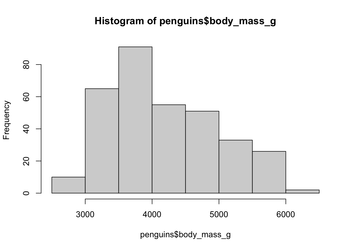
Sometimes it is convenient to adjust the bin width:
hist(penguins$body_mass_g, breaks = 50)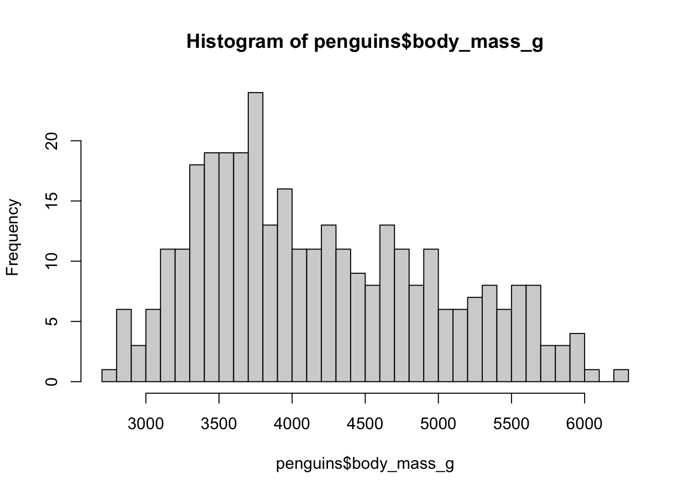
The dataset also contains the measure of flipper lengths. Is there a relationship between this measure and body mass? Use the function plot() which plots a scatter plot of two numeric vectors (both given as x and y parameters of the function — look at ?plot again if needed!) to visualize the relationship between those two variables / columns: penguins$flipper_length_mm against penguins$body_mass_g. Is there an indication of a relationship between the two metrics?
NoteClick to see the solution
Here is the plain scatter plot — there does seem to be a linear relationship indeed, which makes sense! The larger the penguin (body mass) the longer its flippers!
plot(penguins$flipper_length_mm, penguins$body_mass_g)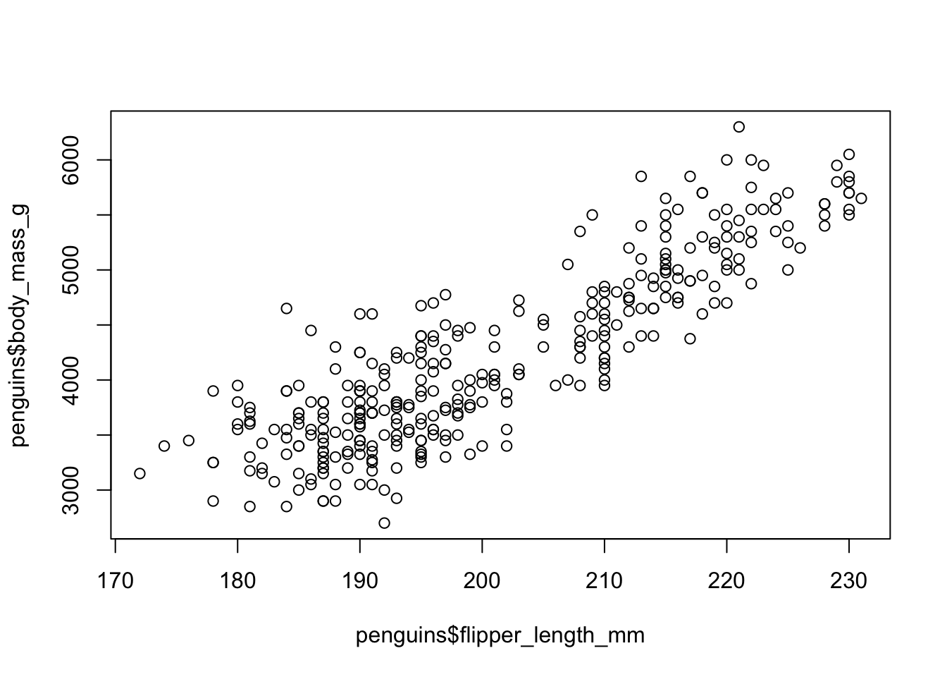
Just for fun, we can also overlay a linear fit (first computed with the lm() function, then visualized as a red dashed line using another built-in function abline():
plot(penguins$flipper_length_mm, penguins$body_mass_g)

lm_fit <- lm(body_mass_g ~ flipper_length_mm, data = penguins)
abline(lm_fit, col = "red", lty = 2)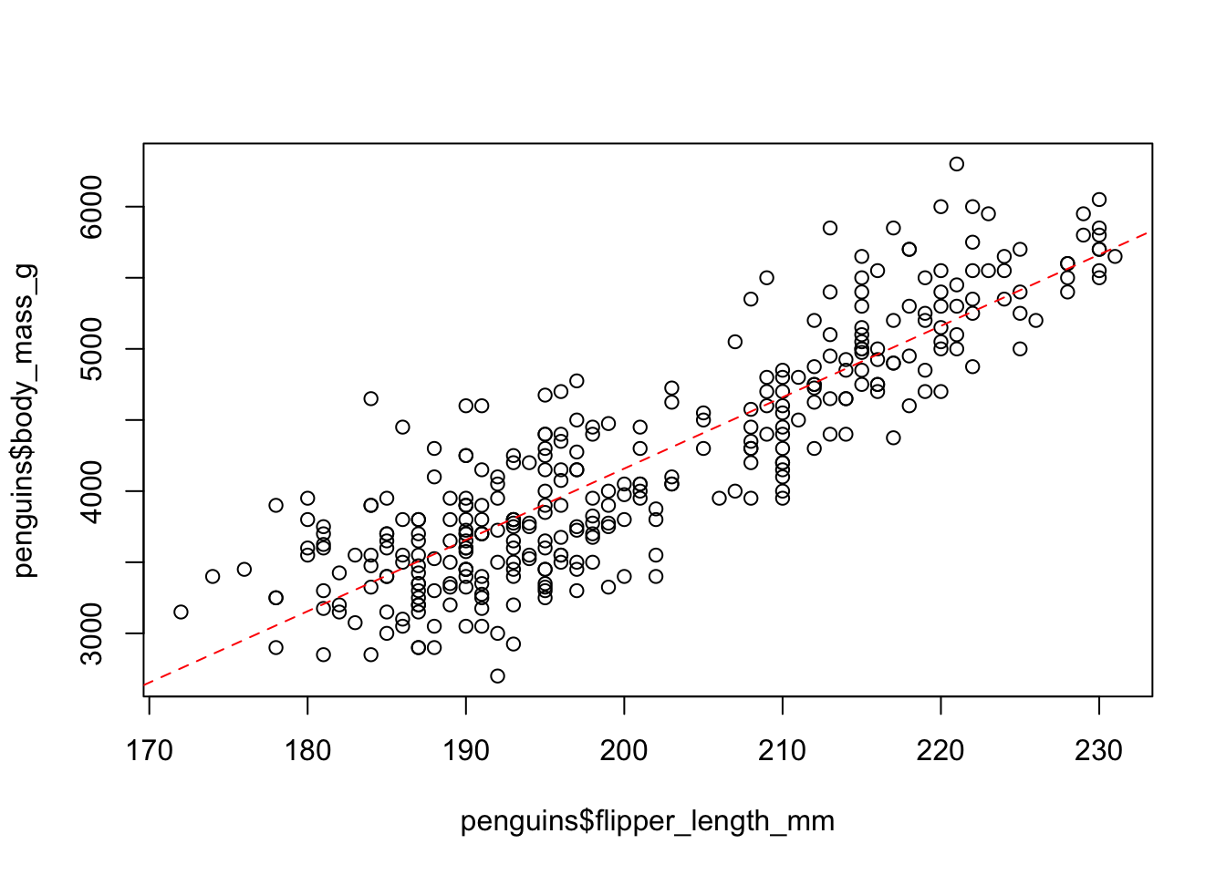
We can also see that we have data for three different species of penguins. We can therefore partition the visualization for each species individually (again, you can always find additional options and examples in help pages such as ?plot):
plot(penguins$flipper_length_mm, penguins$body_mass_g, col = penguins$species)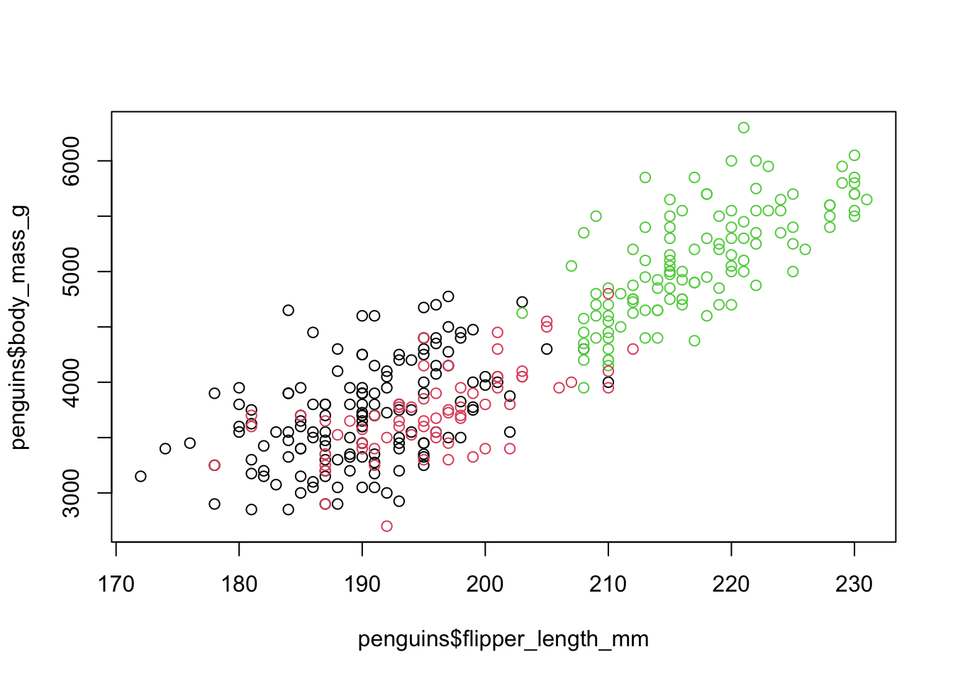
Base R plotting is very convenient for quick and dirty data summaries, particularly immediately after reading unknown data. However, for anything more complex (and anything more pretty), ggplot2 is unbeatable. For this reason, there’s no point in digging into base R graphics any further.
We will be looking at ggplot2 visualization in the session on tidyverse but as a sneakpeak, you can take a look at the beautiful figures you’ll learn how to make later.
NoteSee the sneakpeak
Look how comparatively little code we need to make beautiful informative figures (much prettier than those made with base R functions like we did just above) which immediately tell a clear story! Stay tuned for later! :)
library(ggplot2)
library(dplyr)
Code
ggplot(penguins) +
  geom_histogram(aes(flipper_length_mm, fill = species), alpha = 0.5) +
  theme_minimal() +
  ggtitle("Distribution of flipper lengths across species")
`stat_bin()` using `bins = 30`. Pick better value `binwidth`.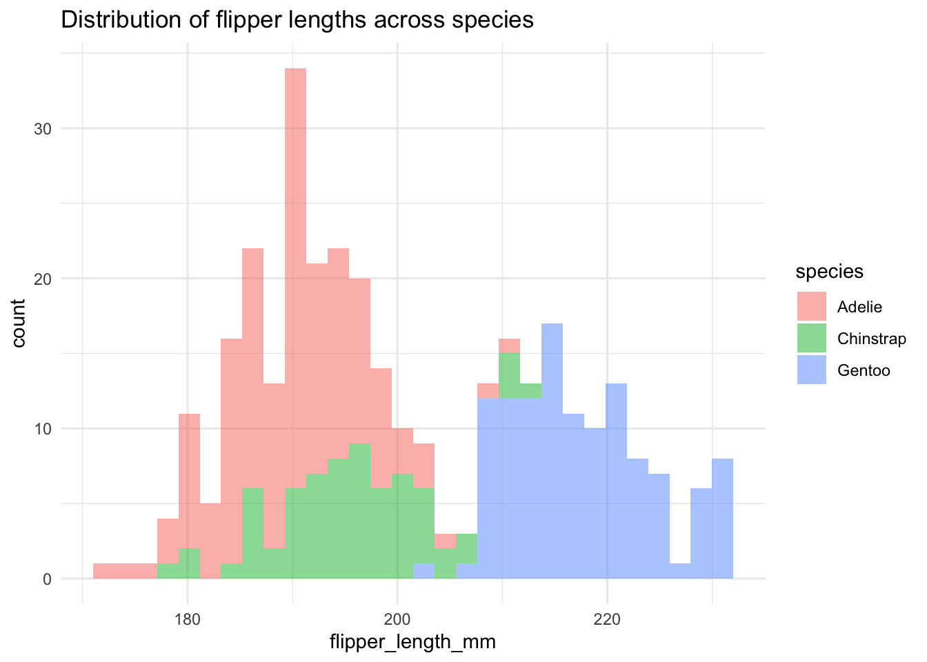
Code
ggplot(penguins, aes(flipper_length_mm, body_mass_g, shape = sex, color = species)) +
  geom_point() +
  geom_smooth(method = "lm") +
  facet_wrap(~ species) +
  theme_minimal() +
  ggtitle("Body mass as a function of flipper length across penguin species")
`geom_smooth()` using formula = 'y ~ x'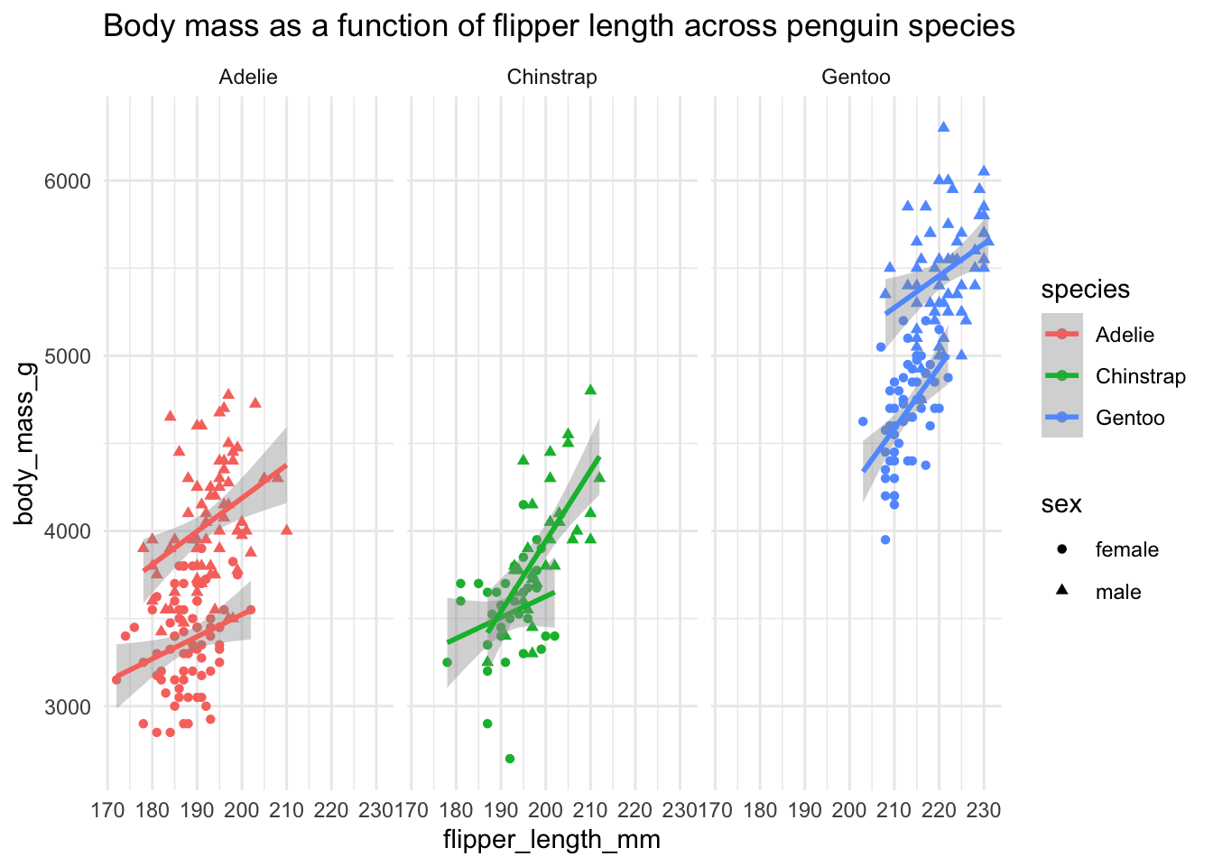
Exercise 9: Working with directories and files
When we move on to the reproducibility session and begin discussing the benefits of writing self-contained, single-purpose R scripts as components of reproducible pipelines, it will come in handy for our scripts to do more than just munge on tables and create plots. Sometimes our scripts will create files. And those files need directories to be put in.
Yes, we can always do this manually in a file explorer of some sorts, but that is not automated and, as a result, it’s not reproducible.
Orienting ourselves
Your R session (where your script lives and where your R console exists) always has an “active directory” in which it is assumed to operate, unless this is changed.
You can always get this by running getwd() (“Get Working Directory”). Where is your R session’s working directory right now?
You can change this directory by executing the command setwd() (“Set Working Directory”).
Both can be useful in automated workflow scripts, which we will get to in later sessions. For now just keep in mind that R gives you a lot of possibilities to work with your filesystem.
Creating a directory
You can create a directory using a function dir.create(). Try it by creating a directory somewhere on your file system, named “testing-directory”. Look up ?dir.create help page to see useful options.
What happens when you call a dir.create("testing-directory") twice? Do you get an error or a warning? Is that warning necessarily a problem, or is it more that it’s annoying? (Imagine having a script which does this repeatedly, perhaps because it can be run repeatedly in a loop). How would you silence this problem? Again, look up the help under ?dir.create.
Listing files
Often you have many different tables stored across multiple files. You then need to read all those tables, but calling a function like read_tsv() (which reads a data frame from disk — we’ll use it a lot in later sections!) a hundred times, manually, is impossible.
A useful trick is to get a listing of files in a particular directory, using the function list.files().
Use list.files() to list all files in your ~/Documents directory. Again, look up help for ?list.files to see how you should run this function. Experiment in your R console! Do you get full paths to each file? Or just filenames? How would you get full paths?
Using list.files() is particularly helpful in conjunction with the concept of looping introduced towards the end of this Bootcamp session.
Don’t worry too much about this technical stuff. When the moment comes that you’ll need it in your project, just refer back to this!
Testing the existence of a directory or a file
In other setting, we need our script to test whether a particular directory (or, more often, a file) already exists. This can be done with the functions dir.exists() or file.exists().
Pick an arbitrary file you got in your ~/Documents listing. Then try file.exists() on that file. Then add a random string to that path to your file and run file.exists() again.
These functions are also super useful for building more comprehensive pipelines! Imagine a situation in which an output file with your results already exists, and you don’t want to overwrite it (but you want to run your script as a whole anyway).
Exercise 10: Functions
The motivation for this Exercise could be summarized by an ancient principle of computer programming known as “Don’t repeat yourself” (DRY) which is present when:
“[…] a modification of any single element of a system does not require a change in other logically unrelated elements.”.
Let’s demonstrate this idea in practice on the most common way this is applied in practice, which is encapsulating (repeatedly used) code in self-contained functions.
Let’s say you have the following numeric vector (these could be base qualities, genotype qualities, \(f\)-statistics, sequencing coverage, anything normally probably stored in a data-frame column, but here represented as a plain numeric vector):
vec <- c(0.32, 0.78, 0.68, 0.28, 1.96, 0.21, 0.07, 1.01, 0.06, 0.74,
         0.37, 0.6, 0.08, 1.81, 0.65, 1.23, 1.28, 0.11, 1.74,  1.68)
With numeric vectors, we often need to compute some summary statistics (mean, median, quartile, minimum, maximum, etc.). What’s more, in a given project, we often have to do this computation multiple times in a number of places.
Note: In R, we have a very useful built-in function summary(), which does exactly that. But let’s ignore this for the moment, for learning purposes.
Here is how you can compute those summary statistics individually:
min(vec)
## [1] 0.06

# first quartile (a value which is higher than the bottom 25% of the data)
quantile(vec, probs = 0.25)
##    25%
## 0.2625

median(vec)
## [1] 0.665

mean(vec)
## [1] 0.783

# third quartile (a value which is higher than the bottom 75% of the data)
quantile(vec, probs = 0.75)
##    75%
## 1.2425

max(vec)
## [1] 1.96
Now, you can imagine that you have many more of such vectors (results for different sequenced samples, different computed population genetic metrics, etc.). Having to type out all of these commands for every single one of those vectors would very quickly get extremely tiresome. Worse still, when we would do this, we would certainly resort to copy-pasting, which is guaranteed to lead to errors.
Custom functions are the best solution to this problem and a key thing most scientists are not aware of which can tremendously improve reproducibility.
How are functions defined
A custom function in R is defined by the following patterns. Note that it looks like a variable definition, except the variable (later refered to as a “function name”, here fun_name) is assigned <- a more complex code structure known as “function” body, with the code enclosed in { and } block delimiters.
Custom functions can take several forms, most importantly:
- The function can be without parameters, defined like this:
fun_name <- function() {
  # here goes your code
}
And then called like this (without parameters, and not returning anything):
fun_name()- Or it can have some parameters, which are variables that are passed to that function (and can be used inside the function like any other variable — here just parameter variables
par1,par2):
fun_name <- function(par1, par2) {
  # here goes your code
}
And then called like this (still not returning anything):
# variable1 will be assigned to par1 inside the function
# variable2 will be assigned to par2 inside the function
fun_name(variable1, variable2) - A function can also return a result, represented by a variable created inside that function, and returned by the
return()statement typically at the end of the function body (but not always):
fun_name <- function(par1, par2) {
  # here goes your code

  # the code could create a variable like this:
  result <- # however you would compute the result

  return(result)
}
And then used like this:
# the returned value from the function is assigned to a variable
# result_from_function which we can work with later
result_from_function <- fun_name(par1, par2)
Spoilers ahead for more advanced researchers
If you’re a more advanced researcher, in the later parts on practical reproducibility techniques, extracting your repetitive code into self-contained, well-documented functions, and putting collections of such functions into independent “utility module” scripts which can be sourced into data analysis scripts using the source() command is the single best, most important thing you can do do increase the robustness and reproducibility of your own projects!
When you find yourself with free time, use these lessons to improve your projects by doing this!
Write a custom function called my_summary, which will accept a single input named values (a vector of numbers like vec above), and return a list which combines all the six summary statistics together. Name the elements of that list as "min", "quartile_1", "median", "mean", "quartile_3", and "max".
Hint: You can use the following “template”, and just fill in the required bits of code within the “function body” represented by { and }:
# copy this template into your script and add relevant bits of code to
# turn it into a full-blown R function

my_summary <- function(values) {
  # compute
  # your
  # summary
  # statistics
  # like
  # you
  # did
  # above

  result <- list(... combine your statistics into a named list as instructed ...)

  # then return that result
  return(result)
}
Then test that your function works correctly by executing it like this in your R console:
my_summary(vec)Yes, we had to write the code anyway, we even had to do the extra work of wrapping it inside other code (the function body, name the one input argument values, which could be multiple arguments for more complex function). So, one could argue that we didn’t actually save any time. However, that code is now “encapsulated” in a fully self-contained form and can be called repeatably, without any copy-pasting.
In other words, if you now create these three vectors of numeric values:
vec1 <- runif(10)
vec2 <- runif(10)
vec3 <- runif(10)
You can now compute our summary statistics by calling our function my_summary() on these vectors, without any code repetition:
The punchline is this: if we ever need to modify how are summary statistics are computed, we only have to make a single change in the function code instead of having to modify multiple copies of the code in multiple locations in our project. This is what “Don’t Repeat Yoursef (DRY)” means!
In the penguin section above, you used hist(penguins$body_mass) to plot a histogram of the penguins’ body mass. Write a custom function penguin_hist() which will accept two arguments: 1. the name of the column in the penguins data frame, and 2. the number of histogram breakpoints to use as the breaks = arguments in a hist(<vector>, breaks = ...) call.
Hint: Remember that you can extract a column of a data frame as a vector not just using a symbolic identifier with the $ operator but also as a string name with the [[]] operator.
Hint: A useful new argument of the hist() function is main =. You can specify this as a string and the contents of this argument will be plotted as the figure’s title.
If you need further help, feel free to use this template and fill the insides of the function body with your code:
penguin_hist <- function(df, column, breaks) {
  # ... put your hist() code here
}
NoteClick to see the solution
We can extract a column column of any data frame df with df[[column]], therefore, we only need to do this:
penguin_hist <- function(df, column, breaks) {
  title <- paste("Histogram of the column", column)
  hist(df[[column]], breaks = breaks, main = title)
}
We can then use our fancy new function like this:
penguin_hist(penguins, "bill_length_mm", breaks = 50)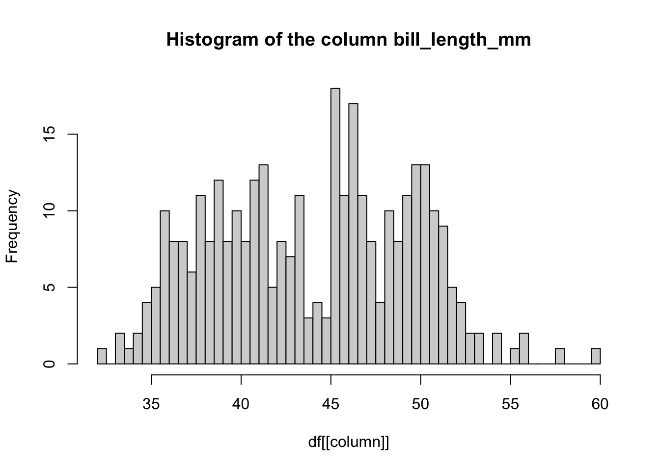
penguin_hist(penguins, "bill_depth_mm", breaks = 50)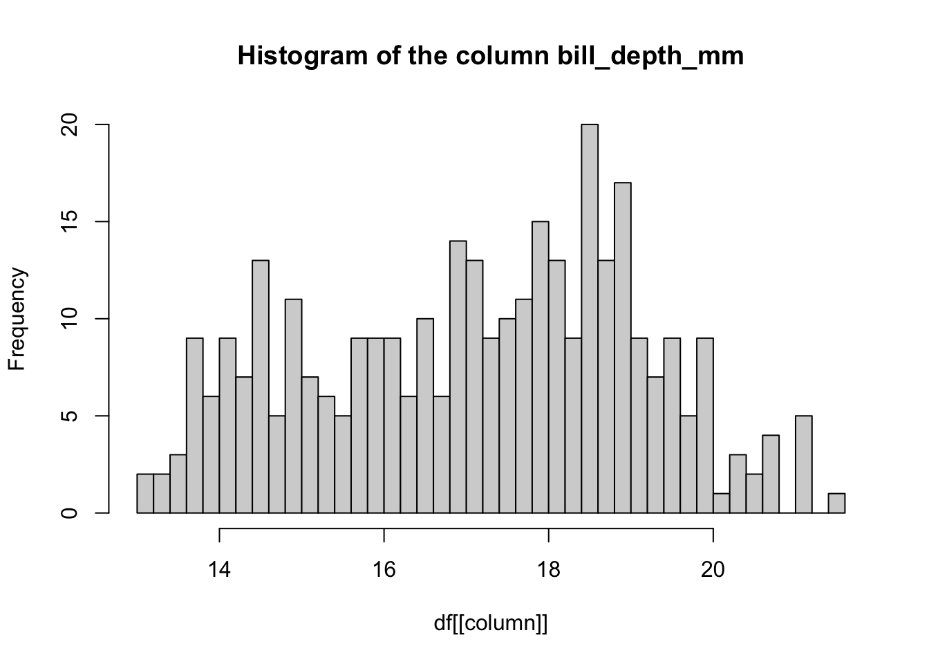
penguin_hist(penguins, "flipper_length_mm", breaks = 50)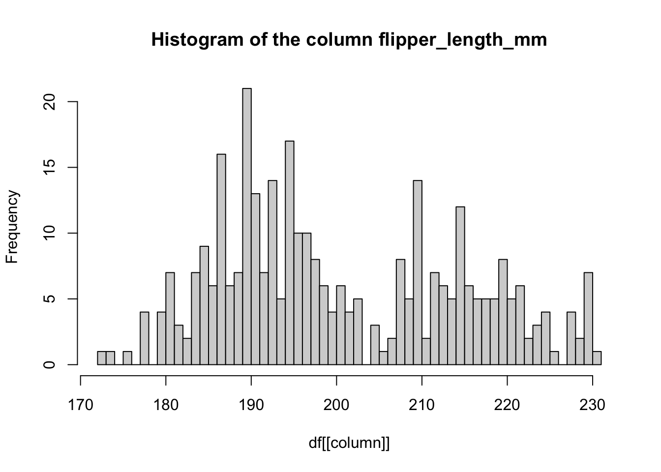
penguin_hist(penguins, "body_mass_g", breaks = 50)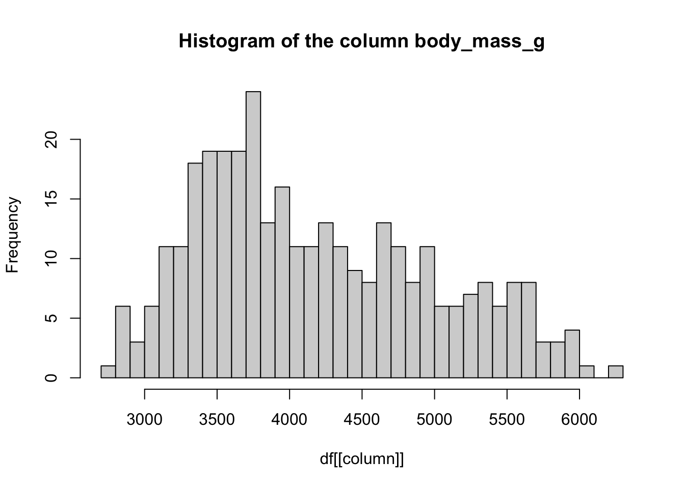
Exercise 11: Conditional expressions
Oftentimes, especially when writing custom code, we need to make automated decisions whether something should or shouldn’t happen given a certain value. We can do this using the if expression which has the following form:
if (<condition resulting in TRUE or FALSE>) {
  ... code which should be executed if condition is TRUE...
}
An extension of this is the if-else expression, taking the following form:
if (<condition resulting in TRUE or FALSE>) {
  ... code which should be executed if condition is TRUE...
} else {
  ... code which should be executed if condition is FALSE...
}
Go back to your new penguin_hist() function and add an if expression which will make sure that breaks is greater than 0. In other words, if breaks < 1 (the condition you will be testing against), execute the command stop("Incorrect breaks argument given!").
This was just a little sneak peak. As you get more comfortable with programming, if and if-else expressions like this will be very useful to make your code more robust. Whenever you’re coding, catching errors as soon as they happen is extremely important!
Exercise 12: Iteration and loops
Functions help us take pieces of code and generalize them to reduce the amount of code needed to do similar things, repeatedly, multiple times, and avoid code duplication by copy-pasting (nearly the same) chunks of code over and over. You could think of iteration as generalizing those repetitions even further. Instead of manually calling a bit of code repeatedly, we can iterate over that code in an iterative way.
In general, there are two types of loops:
1. Loops producing a value for each iteration
The loops in this category which we are going to encounter most often are those of the apply family, like lapply() or sapply(). The general pattern like this:
result <- lapply(<vector/list of values>, <function>)The lapply and sapply functions take, at minimum, a vector or a list as their first argument, and then a function which takes a single argument. Then they apply the given function to each element of the vector/list, and return either a list (if we use the lapply() function) or a vector (if we use the sapply() function).
Let’s consider this more concrete example:
input_list <- list("hello", "this", 123, "is", "a mixed", 42, "list")

result_list <- lapply(input_list, is.numeric)

result_list
[[1]]
[1] FALSE
[[2]]
[1] FALSE
[[3]]
[1] TRUE
[[4]]
[1] FALSE
[[5]]
[1] FALSE
[[6]]
[1] TRUE
[[7]]
[1] FALSEWe took an input_list and applied a function to each element, automatically, gathering the results in another list!
Create the following function which, for a given number, returns TRUE if this number is even and FALSE if the number is odd. Then use sapply() to test which of the following numbers in the input_vector is odd or even. Notice that we can do thousands or even millions of operations like this (for very very long input vectors) with a single sapply() command!
input_vector <- c(23, 11, 8, 36, 47, 6, 66, 94, 20, 2)

is_even <- function(x) {
  x %% 2 == 0 # this answers the question "does x divided by 2 give 0?")
}As a practice of indexing, use the result of the sapply() you just got to filter the input_vector values to only odd numbers.
Hint: Remember that you can negate any TRUE / FALSE value (even vector) using the ! operator.
These examples are perhaps too boring to see immediate usefulness of sapply() and lapply() for real-world applications. In later sessions, we will see more complex (and more useful) applications of these functions in daily data analysis tasks.
That said, you can hopefully see how automating an action of many things at once can be very useful means to save yourself repeated typing of the same command over and over. Again, consider a situation in which you have thousands or even millions of data points!
2. Loops which don’t necessarily return a value
This category of loops most often takes form of a for loop, which generally have the following shape:
for (<item> in <vector or list>) {
  ... some commands ...
}
The most trivial runnable example I could think of is this:
# "input" vector of x values
xs <- c(1, 2, 3, 4, 5, 6, 7, 8, 9, 10)

# take each x out of all given xs in sequence...
for (x in xs) {
  # ... and print it out on a new line
  cat("The square of", x, "is", x^2, "\n")
}
The square of 1 is 1
The square of 2 is 4
The square of 3 is 9
The square of 4 is 16
The square of 5 is 25
The square of 6 is 36
The square of 7 is 49
The square of 8 is 64
The square of 9 is 81
The square of 10 is 100 Note: cat() is a very useful function which prints out a given value (or here, actually, multiple values!). If we append "\n" it will add an (invisible) “new line” character, equivalent of hitting ENTER on your keyboard when writing.
Let’s say you want to automate the plotting of several numeric variables from your penguins data frame to a PDF using your custom-defined function penguin_hist() you created above. Fill in the necessary bits of code in the following template to do this! This is a super common pattern that comes in handy very often in data science work.
Note: You can see the cat() call in the body of the for loop (we call the insides of the { ... } block the “body” of a loop). When you iterate over many things, it’s very useful to print out this sort of “log” information, particularly if the for loop can take very long.
# create an empty PDF file
pdf("penguins_hist.pdf")

# let's define our variables of interest (columns of a data frame)
# ... put your code here ...

# let's now "loop over" each of those variables
for (var in variables) {
# ... put your plotting code here ...
}

dev.off() # this closes the PDFIf everything works correctly, look at the penguins_hist.pdf file you just created! It was all done in a fully automated way! A hugely important thing for reproducibility.
If you want, look up ?pdf to see how you could modify the width and height of the figures that will be created.
Further resources
If you have energy and time, take a look at the following chapters of the freely-available Advanced R textbook (the best resource for R programming out there). First work through the quiz at the beginning of each chapter. If you’re not sure about answers (the questions are very hard, so if you can’t answer them, that’s completely OK), work through the material of each chapter and try to solve the exercises.
Pick whichever topic seems interesting to you. Don’t try to ingest everything – even isolated little bits and details that stick with you will pay off in the long run! I strongly suggest you start with the debugging topic (particularly the interactive debugging features of R and RStudio) because this will have the biggest immediate impact on your own work.