library(slendr)
init_env()

simulate_afs <- function(Ne) {
  # In here you should write code which will:
  #   1. create one population with a given Ne (provided as a function argument)
  #   2. compile a model using `simulation_length =` and `generation_time =`
  #   3. simulate a tree sequence
  #   4. select names of 10 samples (doesn't matter which, "pop_1", "po2_", ...)
  #   5. compute AFS vector from those 10 individuals using `ts_afs()`

  # `result` is a variable with your 10-sample AFS vector (we remove the
  # first element because it's not meaningful for our example)
  return(result[-1])
}

afs_1 <- simulate_afs(Ne = 1000) # simulate AFS from a Ne = 1000 model...
plot(afs_1, type ="o") # ... and plot it\(N_e\) inference with AFS
So far we’ve learned how slendr provides an easy way to define demographic models in R and simulate (even very large!) tree sequences from them. This allows us to quickly verify our intuition about some popgen problem (things like “Hmmm, I wonder what would an \(f_4\) statistic look like if my model includes this particular gene-flow event?), in just a few lines of R. There have been instances in which we’ve been able to even answer questions like this directly in a meeting, pretty much on the spot! This makes slendr a very powerful “popgen calculator”.
Now let’s take things one step further. Imagine you gathered some empirical data, like an allele frequency spectrum (AFS) from a population that you study. That data was, in the real world, produced by some (hidden) biological process (demographic history) that we want to learn about. For instance, the population we study had some \(N_e\), which we don’t know the value of (the only thing we have is the observed AFS) but we want to infer that value.
Simulations can be a great tool to estimate the most likely value of such an unknown parameter. Briefly speaking, in this particular toy example, we can simulate a large number of AFS vectors (each resulting from a different assumed \(N_e\) value) and then pick just those \(N_e\) values (or just one \(N_e\) value) which produced a simulated AFS closest to the observed AFS.
This is exactly what you’ll be doing just now.
Exercise 1: A self-contained slendr function of \(N_e \rightarrow \textrm{AFS}\)
In a new script inference-afs.R write a custom R function called simulate_afs(), which will take Ne as its only parameter. Use this function to compute (and return) AFS vectors for a couple of Ne values of your choosing, but staying between Ne = 1000 and Ne = 30000 Plot those AFS vectors and observe how (and why?) do they differ based on Ne parameter you used in each respective simulation.
Hint: The function should create a one-population forward-time model (our population starting at time = 1, with the model simulation_length = 100000 and generation_time = 1 in compile_model()), simulate 10Mb tree sequence using msprime() (recombination rate 1e-8) and then overlay neutral mutations on it at mutation_rate = 1e-8), compute AFS for 10 samples and return the AFS vector as result of this custom function.
Hint: If you’ve never programmed before, the concept of a “custom function” might be very alien to you. Again, if you need help, feel free to start building your inference-afs.R solution based on this “template” (just fill in missing relevant bits of slendr code that you should be already familiar with):
Note: Remember that you should drop the first element of the AFS vector produced by ts_afs() (for instance with something like result[-1] if result contains the output of ts_afs()) technical reasons related to tskit. You don’t have to worry about that here, but you can read this for more detail.
Hint: If the above still doesn’t make any sense to you, feel free to copy-paste the function from the solution below into your script and work with that function instead!
When used in R, your custom function should work like this (the simulation is stochastic, so your numbers will be different, of course):
# This gives us a vector of singletons, doubletons, etc., etc., all the way
# to the number of fixed mutations in our sample of 10 individuals
simulate_afs(Ne = 1000)
[1] 382 201 126 102 74 44 48 60 32 35 29 32 30 21 22 26 40 36 21
[20] 34
NoteClick to see the solution
A function can be understood as a independent unit of a computer program which executes a block of code inside the {…} brackets given some values of some parameters. In our example, we programmed a function simulate_sfs() which accepts a single parameter, Ne.
simulate_afs <- function(Ne) {
  # create a slendr model with a single population of size Ne = N
  pop <- population("pop", N = Ne, time = 1)
  model <- compile_model(pop, generation_time = 1, simulation_length = 100000)

  # simulate a tree sequence
  ts <-
    msprime(model, sequence_length = 10e6, recombination_rate = 1e-8) %>%
    ts_mutate(mutation_rate = 1e-8)

  # get a random sample of names of 10 individuals
  samples <- ts_names(ts) %>% sample(10)

  # compute the AFS vector (dropping the 0-th element added by tskit)
  afs <- ts_afs(ts, sample_sets = list(samples))[-1]

  afs
}
Our functions is supposed to produce an AFS vector of counts of alleles observed at a given frequency a the population sample:
Let’s use our custom function to simulate AFS vector for Ne = 1k, 10k, and 30k:
afs_1k <- simulate_afs(1000)
afs_10k <- simulate_afs(10000)
afs_30k <- simulate_afs(30000)
Here’s one of those vectors. We can see that the function does, indeed, produce a result of the correct format:
afs_1k [1] 399 184 147 103 66 66 41 30 50 28 51 35 28 22 22 33 32 22 28
[20] 29To see the results of this function in a clearer context, let’s visualize the vectors in the same plot:
plot(afs_30k, type = "o", main = "AFS, Ne = 30000", col = "cyan",)
lines(afs_10k, type = "o", main = "AFS, Ne = 10000", col = "purple")
lines(afs_1k, type = "o", main = "AFS, Ne = 1000", col = "blue")
legend("topright", legend = c("Ne = 1k", "Ne = 10k", "Ne = 30k"),
       fill = c("blue", "purple", "cyan"))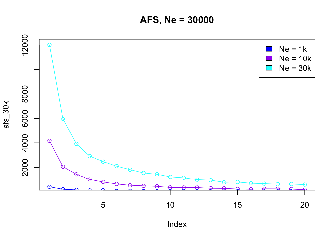
Exercise 2: Estimating unknown \(N_e\) from empirical AFS
Imagine you sequenced 10 samples from a population and computed the following AFS vector (which contains, sequentially, the number of singletons, doubletons, etc., in your sample from a population):
afs_observed <- c(2520, 1449, 855, 622, 530, 446, 365, 334, 349, 244,
                  264, 218,  133, 173, 159, 142, 167, 129, 125, 143)
You know (maybe from some fossil evidence) that the population probably had a constant \(N_e\) somewhere between 1000 and 30000 for the past 100,000 generations, and had mutation and recombination rates of 1e-8 (i.e., parameters already implemented by your simulate_afs() function – how convenient!).
Use slendr simulations to guess the true (and hidden!) \(N_e\) given the observed AFS by running simulations for a range of \(N_e\) values and finding out which \(N_e\) produces the closest AFS vector to the afs_observed vector above using one of the following two approaches.
Option 1 [easy]: Plot AFS vectors for various \(N_e\) values (i.e. simulate several of them using your function
simulate_afs()), then eyeball which looks closest to the observed AFS based on the figures alone. (This is, of course, not how proper statistical inference is done, but it will be good enough for this exercie!)Option 2 [hard]: Simulate AFS vectors in steps of possible
Ne(maybelapply()?), and find the \(N_e\) which gives the closest AFS to the observed AFS based on Mean squared error.
NoteClick to see the solution to “Option 1”
This is the observed AFS with which we want to compare our simulated AFS vectors:
afs_observed <- c(2520, 1449, 855, 622, 530, 446, 365, 334, 349, 244,
                  264, 218,  133, 173, 159, 142, 167, 129, 125, 143)
We know that the true \(N_e\) is supposed to be between 1000 and 30000, so let’s simulate a bunch of AFS vectors for different \(N_e\) values using our new AFS simulation function:
afs_Ne1k <- simulate_afs(Ne = 1000)
afs_Ne5k <- simulate_afs(Ne = 5000)
afs_Ne6k <- simulate_afs(Ne = 6000)
afs_Ne10k <- simulate_afs(Ne = 10000)
afs_Ne20k <- simulate_afs(Ne = 20000)
afs_Ne30k <- simulate_afs(Ne = 30000)
Now let’s plot our simulated AFS vectors together with the observed AFS (highlighting it in black):
plot(afs_observed, type = "b", col = "black", lwd = 3,
     xlab = "allele count bin", ylab = "count", ylim = c(0, 13000))
lines(afs_Ne1k, lwd = 2, col = "blue")
lines(afs_Ne5k, lwd = 2, col = "green")
lines(afs_Ne6k, lwd = 2, col = "pink")
lines(afs_Ne10k, lwd = 2, col = "purple")
lines(afs_Ne20k, lwd = 2, col = "orange")
lines(afs_Ne30k, lwd = 2, col = "cyan")
legend("topright",
       legend = c("observed AFS", "Ne = 1000", "Ne = 5000",
                  "Ne = 6000", "Ne = 10000", "Ne = 20000", "Ne = 30000"),
       fill = c("black", "blue", "green", "pink", "purple", "orange", "cyan"))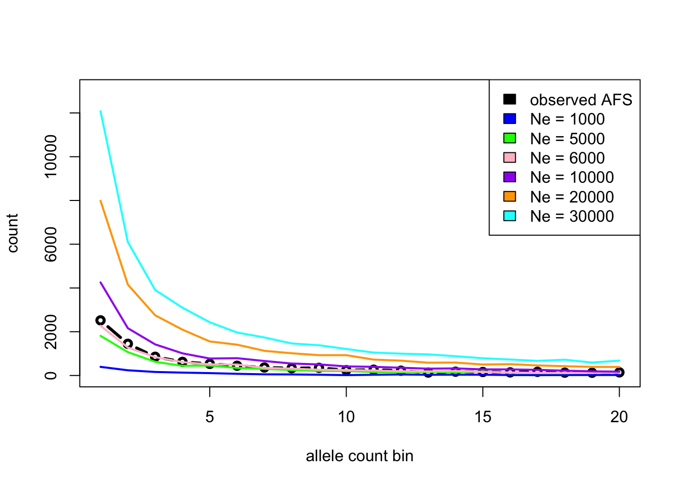
The true \(N_e\) was 6543!
NoteClick to see the solution to “Option 2”
This is the observed AFS with which we want to compare our simulated AFS vectors:
afs_observed <- c(2520, 1449, 855, 622, 530, 446, 365, 334, 349, 244,
                  264, 218,  133, 173, 159, 142, 167, 129, 125, 143)
We know that the true \(N_e\) is supposed to be between 1000 and 30000. Let’s generate regularly spaced values of potential Ne values whose AFS we want to investigate and compare to the obesrved AFS (our parameter grid):
Ne_grid <- seq(from = 1000, to = 30000, by = 500)
Ne_grid
[1] 1000 1500 2000 2500 3000 3500 4000 4500 5000 5500 6000 6500
[13] 7000 7500 8000 8500 9000 9500 10000 10500 11000 11500 12000 12500
[25] 13000 13500 14000 14500 15000 15500 16000 16500 17000 17500 18000 18500
[37] 19000 19500 20000 20500 21000 21500 22000 22500 23000 23500 24000 24500
[49] 25000 25500 26000 26500 27000 27500 28000 28500 29000 29500 30000With the parameter grid Ne_grid set up, let’s simulate an AFS from each \(N_e\) model:
library(parallel)

afs_grid <- mclapply(Ne_grid, simulate_afs, mc.cores = detectCores())
names(afs_grid) <- Ne_grid

# show the first five simulated AFS vectors, for brevity, just to demonstrate
# what the output of the grid simulations is supposed to look like
afs_grid[1:5]
$`1000`
[1] 463 234 138 90 72 78 48 36 34 31 31 13 33 42 29 19 15 14 20
[20] 40
$`1500`
[1] 541 267 190 142 105 91 58 75 51 55 48 29 51 43 55 24 32 27 28
[20] 46
$`2000`
[1] 889 412 285 244 154 146 135 89 122 97 92 52 73 43 51 62 73 45 31
[20] 41
$`2500`
[1] 1031 524 350 263 165 217 139 114 115 87 96 66 66 79 40
[16] 76 73 56 68 34
$`3000`
[1] 1248 639 423 242 210 192 170 188 158 131 119 105 69 99 78
[16] 77 58 63 47 45Plot the observed AFS and overlay the simulated AFS vectors on top of it:
plot(afs_observed, type = "b", col = "black", lwd = 3, xlab = "allele count bin", ylab = "count")
for (i in seq_along(Ne_grid)) {
  lines(afs_grid[[i]], lwd = 0.5)
}
legend("topright", legend = c("observed AFS", "simulated AFS"), fill = c("black", "gray"))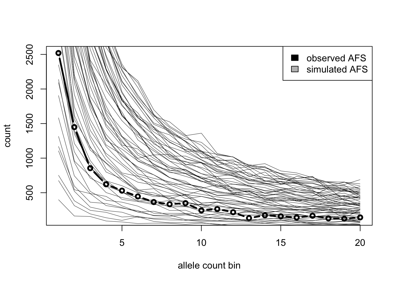
Compute mean-squared error of the AFS produced by each \(N_e\) value across the grid:
errors <- sapply(afs_grid, function(sim_afs) {
  sum((sim_afs - afs_observed)^2) / length(sim_afs)
})

plot(Ne_grid, errors, ylab = "error")
abline(v = Ne_grid[which.min(errors)], col = "red")
legend("topright", legend = paste("minimum error Ne =", Ne_grid[which.min(errors)]), fill = "red")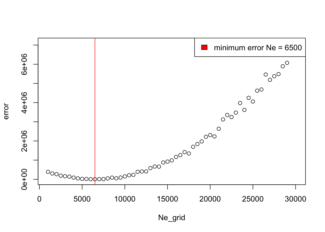
Plot the AFS again, but this time highlight the most likely spectrum (i.e. the one which gave the lowest RMSE value):
plot(afs_observed, type = "b", col = "black", lwd = 3, xlab = "allele count bin", ylab = "count")
for (i in seq_along(Ne_grid)) {
  color <- if (i == which.min(errors)) "red" else "gray"
  width <- if (i == which.min(errors)) 2 else 0.75
  lines(afs_grid[[i]], lwd = width, col = color)
}
legend("topright", legend = c("observed AFS", paste("best fitting Ne =", Ne_grid[which.min(errors)])),
       fill = c("black", "red"))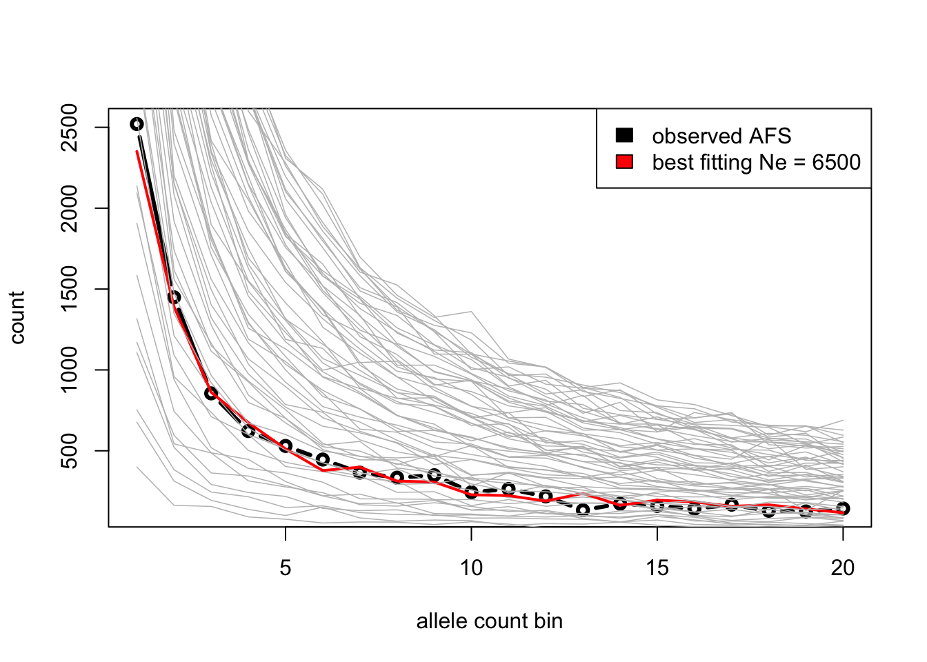
The true \(N_e\) was 6543!
Congratulations, you now know how to infer parameters of evolutionary models using simulations! What you just did is really very similar to how simulation-based inference is done in practice (even with methods such as ABC). Hopefully you now also see how easy slendr makes it to do this (normally a rather laborious) process.
This kind of approach can be used to infer all sorts of demographic parameters, even using other summary statistics that you’ve also learned to compute… including selection parameters, which we delve into in another exercise.