simulate_trajectory <- function(p_init, Ne, generatinos) {
  # ...
  # here is where you will put your code
  # ...
}Algorithmic thinking
⚠️⚠️⚠️ This chapter is a work-in-progress! ⚠️⚠️⚠️
Part XYZ: Generalizing code as a function
You now have all the individual pieces to construct a vector of allele frequency trajectories of a given length (one number in that vector corresponding to one generation of a simulation). Write a function simulate_trajectory(), which will accept the following three parameters and returns the trajectory vector as its output.
p_init: initial allele frequencygenerations: number of generations to simulateNe: effective population size
Then simulate three trajectories with the same parameters (p_init = 0.5, generations = 1000, Ne = 1000 – save them in variables traj1, traj2, traj3) and visualize them on a single plot using the functions plot() and lines() just as we did earlier.
Yes, this basically involves taking the code you have already written and just wrapping it up in a self-contained function!
NoteClick to see the solution
simulate_trajectory <- function(p_init, Ne, generations) {
  trajectory <- c(p_init)

  # for each generation...
  for (gen in seq_len(generations - 1)) {
    # ... based on the allele frequency in the current generation...
    p_current <- trajectory[gen]
    # ... compute the frequency in the next generation...
    n_next <- rbinom(Ne, 1, p_current)
    p_next <- sum(n_next) / Ne
    # ... and save it in the trajectory vector
    trajectory[gen + 1] <- p_next
  }

  return(trajectory)
}

traj1 <- simulate_trajectory(p_init = 0.5, Ne = 1000, generations = 1000)
traj2 <- simulate_trajectory(p_init = 0.5, Ne = 1000, generations = 1000)
traj3 <- simulate_trajectory(p_init = 0.5, Ne = 1000, generations = 1000)

plot(traj1, type = "l", xlim = c(1, 1000), ylim = c(0, 1), xlab = "generations", ylab = "allele frequency")
lines(traj2)
lines(traj3)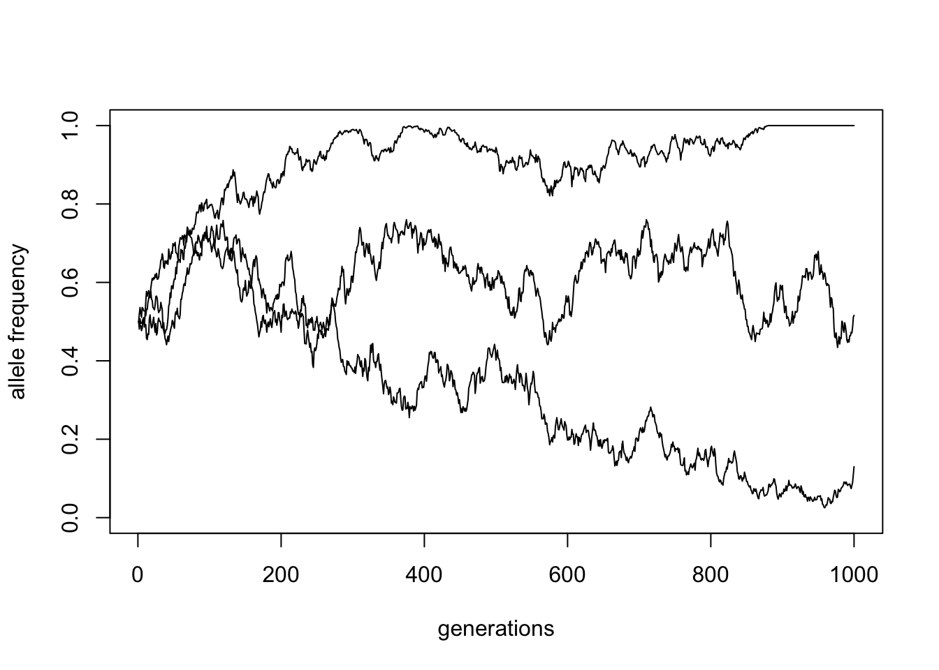
Note: The lines() function will not do anything on its own. You use it to add elements to an already exiting figure.
Part XYZ: Return result as a data frame
Now, this one will probably not make much sense now but let’s do this as a practice, for the time being. Modify the simulate_trajectory() function to return a data frame with the following format (this shows just the first five rows). In other words:
- the column
timegives the time at which the frequency was simulated - the column
frequencycontains the simulated vector, (basically, the index of the for loop iteration), p_init_andNeindicate the parameters of the simulation run (and are, therefore, constant for all rows).
| p_init | Ne | time | frequency |
|---|---|---|---|
| 0.5 | 1000 | 1 | 0.500 |
| 0.5 | 1000 | 2 | 0.514 |
| 0.5 | 1000 | 3 | 0.506 |
| 0.5 | 1000 | 4 | 0.499 |
| 0.5 | 1000 | 5 | 0.492 |
Hint: Remember to use the tibble() function to create your data frame (you will need to first load the tibble R package with library(tibble)!), not the default data.frame() function. This will make your life significantly easier.
Note: It might seem super redundant to drag the repeated p_init and Ne, columns in the table, compared to the previous solution of just returning the numeric vector. Of course, which option is better depends on the concrete situation. In this case, the reason for tracking all this “metadata” along with the frequency vector will become clearer later.
Part XYZ: Running simulations in a loop
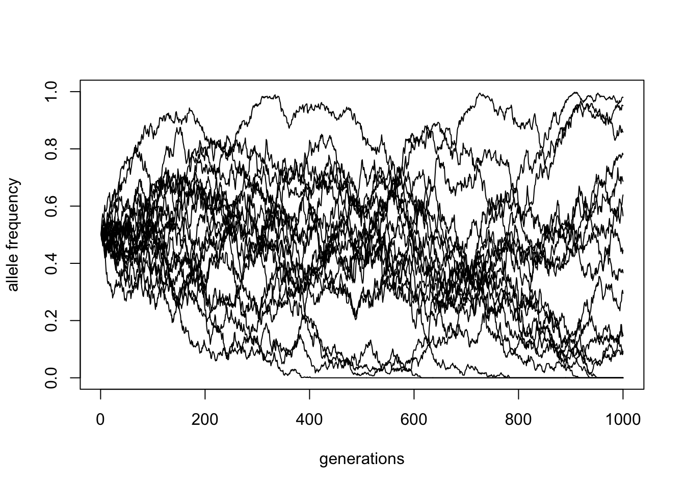
You have now generalized your code so that it is much more flexible by accepting parameters as function inputs. Let’s utilize this self-contained function to run 20 simulations using the function lapply (getting 20 vectors saved in a list in a variable traj_list) and then plot the results by looping over each vector of traj_list in a for loop.
Hint: You can first initialize an empty plot by calling this bit of code:
plot(NULL, type = "l", xlim = c(1, 1000), ylim = c(0, 1),
     xlab = "generations", ylab = "allele frequency")
This basically sets up the context for all trajectories, which you can then plot in the for loop by calling something like lines(<variable>) in the loop body.
NoteClick to see the solution
# run 20 replicates of the simulation
replicates <- 20

simulations <- lapply(
  1:replicates,
  function(i) simulate_trajectory(p_init = 0.5, generations = 1000, Ne = 1000)
)

# create an empty plot (we have to specify the boundaries and other parameters!)
plot(NULL, type = "l", xlim = c(1, 1000), ylim = c(0, 1), xlab = "generations", ylab = "allele frequency")

# then overlay all trajectories in a loop
for (df in simulations) {
  lines(df$frequency)
}