library(slendr)
init_env()Multi-population statistics
Exercise: controlling stochasticity
ts_replicate(
  10,
  {
    ts <-
      msprime(model, sequence_length = 1e6, recombination_rate = 1e-8) %>%
      ts_mutate(mutation_rate = 1e-8)
    pi_df <- ts_diversity(ts, ts_names(ts))
    pi_df$Ne <- pi_df$diversity / (4 * 1e-8)
    pi_df
  }
)
Exercise: Recap on R lists and vectors
Let’s start by doing a bit of a setup. Every time you’ll want to compute some population genomic measure with slendr on your simulated data (\(f4\)-statistic, Tajima’s D, IBD segments, or any of the many others), you will need a way to refer to entities to compute on. The way we do this with slendr is by referring to individual names.
Start by adding this to your script. The variable samples will be used to refer to individuals, define subsets, etc.
samples <- ts_names(ts, split = TRUE)Now let’s work on a couple of basic vector- and list-based operations in R, which we will be using all the time. If you need a recap, you can scroll through the introductory “R bootcamp” chapter, particularly sections and exercises relevant for subsetting and indexing into vectors and lists in R.
What is the type of the data stored in the samples variable? How is the output of ts_names(ts) different from ts_names(ts, split = TRUE)? How many names of individuals does it contain?
Our samples variable contains a vector of the type "character", but it is stored. As of now, it contains the names of length(samples) individuals. TODO
class(samples)samples$p1samples["p1"]samples[["p1"]]“Outgroup” \(f_3\)
Note: The \(f_3\) statistic is traditionally expressed as \(f_3(A, B; C)\), where C represents the outgroup. Unfortunately, in tskit the outgroup is named A, with B and C being the pair of samples from which we trace the length of branches towards the outgroup, so the statistic is interpreted as \(f_3(B, C; A).\)
library(slendr)
init_env()

library(dplyr)   # manipulating tabular data
Attaching package: 'dplyr'The following objects are masked from 'package:stats':
filter, lagThe following objects are masked from 'package:base':
intersect, setdiff, setequal, unionlibrary(ggplot2) # data visualization
library(purrr) # convenient looping functionsWhenever we want to evaluate the behavior of some statistic of interest under a range of demographic scenarios and across different model parameters, it’s always useful to first establish a skeleton structure with concrete values of model parameters, before we wrap it in a dedicated function.
Let’s do this here too.
tsplit <- 5000
outgroup <- population("outgroup", N = 1000, time = 10000)
X <- population("X", N = 1000, time = tsplit, parent = outgroup)
Y <- population("Y", N = 1000, time = tsplit, parent = outgroup)
model <- compile_model(list(outgroup, X, Y), generation_time = 1)
plot_model(model, order = c("outgroup", "X", "Y"), proportions = TRUE)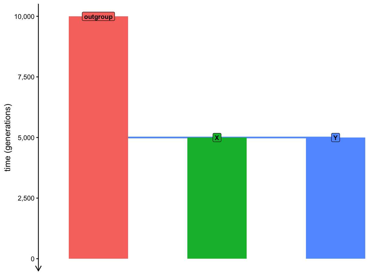
compute_outgroup_f3 <- function(tsplit) {
outgroup <- population("outgroup", N = 1000, time = 10000)
X <- population("X", N = 1000, time = tsplit, parent = outgroup)
Y <- population("Y", N = 1000, time = tsplit, parent = outgroup)
model <- compile_model(list(outgroup, X, Y), generation_time = 1)
ts <- msprime(model, sequence_length = 10e6, recombination_rate = 1e-8) %>% ts_mutate(mutation_rate = 1e-8)
samples <- ts_names(ts, split = TRUE)
ts_f3(ts, A = samples["outgroup"], B = samples["X"], C = samples["Y"]) %>% mutate(tsplit = tsplit)
}compute_outgroup_f3(tsplit = 1000)# A tibble: 1 × 5
A B C f3 tsplit
<chr> <chr> <chr> <dbl> <dbl>
1 outgroup X Y 0.0000122 1000compute_outgroup_f3(tsplit = 2000)# A tibble: 1 × 5
A B C f3 tsplit
<chr> <chr> <chr> <dbl> <dbl>
1 outgroup X Y 0.0000219 2000compute_outgroup_f3(tsplit = 5000)# A tibble: 1 × 5
A B C f3 tsplit
<chr> <chr> <chr> <dbl> <dbl>
1 outgroup X Y 0.0000476 5000f3_outgroup <- map_dfr(seq(1, 10000, by = 1000), compute_outgroup_f3)head(f3_outgroup)# A tibble: 6 × 5
A B C f3 tsplit
<chr> <chr> <chr> <dbl> <dbl>
1 outgroup X Y 0.0000000177 1
2 outgroup X Y 0.0000102 1001
3 outgroup X Y 0.0000191 2001
4 outgroup X Y 0.0000316 3001
5 outgroup X Y 0.0000417 4001
6 outgroup X Y 0.0000490 5001ggplot(f3_outgroup, aes(tsplit, f3)) +
geom_point() +
geom_smooth(method = "lm", se = FALSE, linewidth = 0.5) +
geom_hline(yintercept = 0, linetype = "dashed") +
coord_cartesian(xlim = c(0, 10000))`geom_smooth()` using formula = 'y ~ x'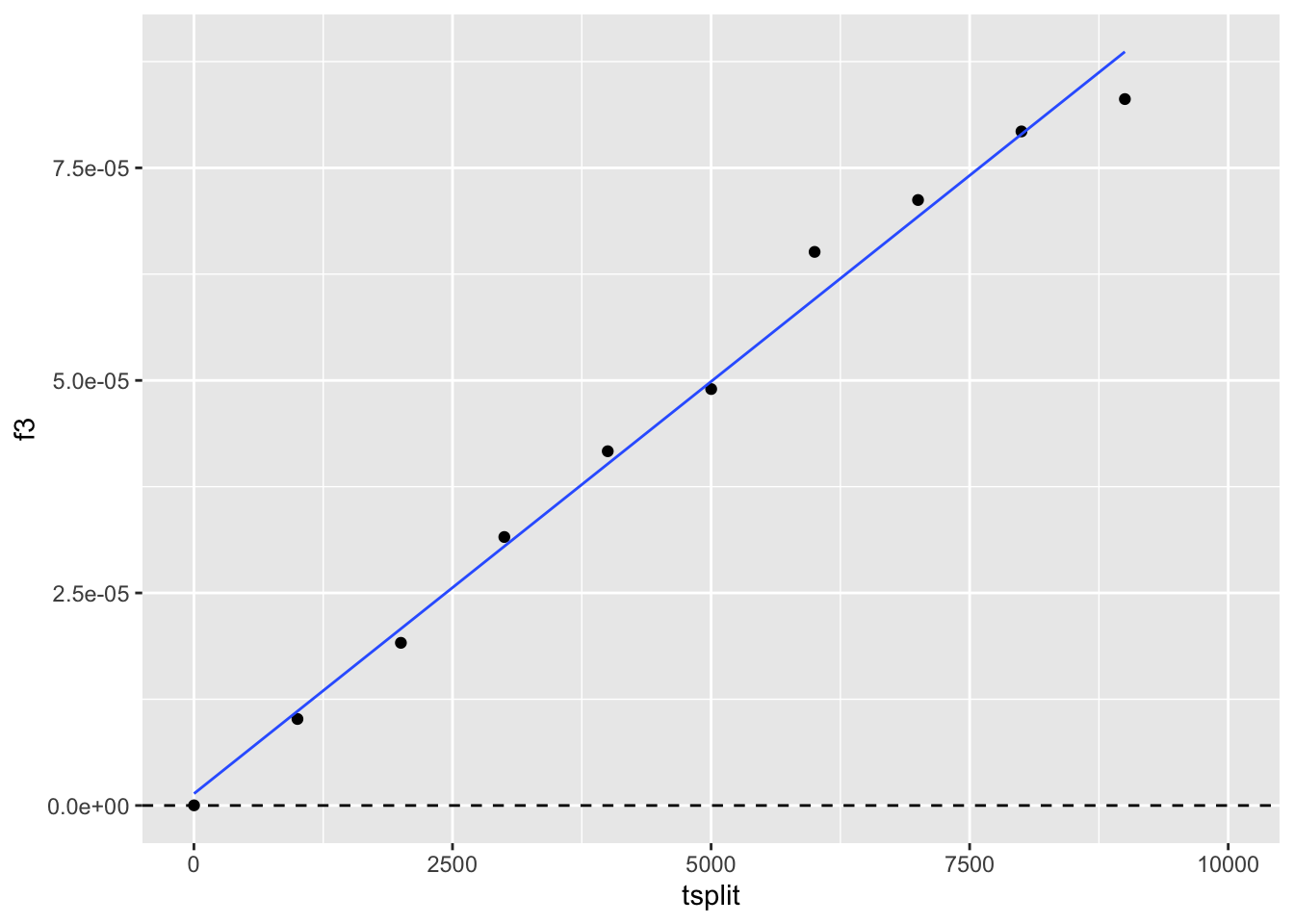
Exercise: mode = "branch" vs mode = "site"
Repeat the exercise 3 by setting mode = "site" in the ts_f3() function calls (this is actually the default behavior of all slendr tree-sequence based tskit functions). This will switch the tskit computation to using mutation counts along each branch of the tree sequence, rather than using branch length themselves. Why might the branch-based computation be a bit better if what we’re after is investigating the expected values of statistics under some model?
Exercise: \(f_3\) statistic as a linear combination of \(f_2\) statistics
You might have learned that any complex \(f\)-statistic can be expressed as a linear combination of multiple \(f_2\) statistics (which represent simple branch length separating two lineages). Verify that this is the case by looking up equation (20b) in this amazing paper and computing an \(f_3\) statistic for any arbitrary trio of individuals of your choosing using such linear combination of \(f_2\) statistics.
Hint: Here’s that equation in a schematic form
f3(A, B; C) = f2(A, C) + f2(B, C) - f2(A, B) / 2Exercise: \(F_{ST}\) losing power with \(N_e\)
“Admixture” \(f_3\)
Now let’s explore the application of the \(f_3\) statistic in its other common use, which is an admixture test. To do this, you will need to expand our baseline population model a little bit.
In our model, we still keep the population outgroup, but the X and Y population now merge at a time tmix to form a population mix. Note that due to the way in which slendr currently implements population merges, you will first need to program the split of mix from X at time tmix - 1, followed at time tmix (i.e., immediately in the following generation) by admixture from U at some defined proportion proportion. To approximate the idea of a population merge as closely as possible within the constraints of the slendr interface, program this admixture event so that it ends after a single generation (i.e., it should end at time tmix + 1).
library(slendr)
init_env()
library(dplyr) # manipulating tabular data
library(ggplot2) # data visualization
library(purrr) # convenient looping functionstmix <- 2000
prop <- 0.1
Ne <- 5000
outgroup <- population("outgroup", N = 5000, time = 10000)
x <- population("x", N = 5000, time = 5000, parent = outgroup)
y <- population("y", N = 5000, time = 5000, parent = outgroup)
mix <- population("mix", N = Ne, time = tmix + 1, parent = x)
gf <- gene_flow(from = y, to = mix, start = tmix, end = tmix - 1, proportion = prop)
model <- compile_model(list(outgroup, x, y, mix), gene_flow = gf, generation_time = 1)
plot_model(model, order = c("outgroup", "x", "mix", "y"), proportions = TRUE)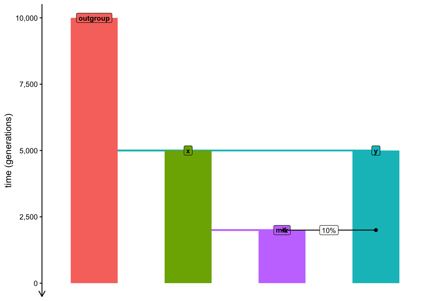
Exercise
Before we start digging into the limitations of the \(f_3\) statistic as a metric for admixture detection, let’s first create a self-contained function which generalizes our baseline model across three main parameters of interest: the admixture time tmix, the admixture proportion prop, and the effective population size of the admixed population Ne:
compute_admix_f3 <- function(tmix, prop, Ne) {
  outgroup <- population("outgroup", N = 5000, time = 10000)
  x <- population("x", N = 5000, time = 5000, parent = outgroup)
  y <- population("y", N = 5000, time = 5000, parent = outgroup)
  mix <- population("mix", N = Ne, time = tmix + 1, parent = x)

  gf <- gene_flow(from = y, to = mix, start = tmix, end = tmix - 1, proportion = prop)

  model <- compile_model(list(outgroup, x, y, mix), gene_flow = gf, generation_time = 1)

  schedule <- schedule_recording(model, times = 0, list(x, 5), list(y, 5), list(mix, 25))

  ts <- msprime(model, sequence_length = 25e6, recombination_rate = 1e-8, schedule = schedule) %>% ts_mutate(mutation_rate = 1e-8)

  samples <- ts_names(ts, split = TRUE)

  ts_f3(ts, A = samples["mix"], B = samples["x"], C = samples["y"]) %>% mutate(tmix = tmix, prop = prop, Ne = Ne)
}compute_admix_f3(tmix = 2000, prop = 0.2, Ne = 10000)# A tibble: 1 × 7
A B C f3 tmix prop Ne
<chr> <chr> <chr> <dbl> <dbl> <dbl> <dbl>
1 mix x y 0.00000125 2000 0.2 10000compute_admix_f3(tmix = 1000, prop = 0.2, Ne = 10000)# A tibble: 1 × 7
A B C f3 tmix prop Ne
<chr> <chr> <chr> <dbl> <dbl> <dbl> <dbl>
1 mix x y -0.00000627 1000 0.2 10000compute_admix_f3(tmix = 1, prop = 0.2, Ne = 10000)# A tibble: 1 × 7
A B C f3 tmix prop Ne
<chr> <chr> <chr> <dbl> <dbl> <dbl> <dbl>
1 mix x y -0.0000144 1 0.2 10000f3_tmix1 <- map_dfr(seq(1, 1500, by = 100), compute_admix_f3, prop = 0.2, Ne = 5000)ggplot(f3_tmix1, aes(tmix, f3)) +
geom_point() +
geom_hline(yintercept = 0, linetype = "dashed") +
geom_smooth(method = "lm", se = FALSE, color = "black", linewidth = 0.5) +
coord_cartesian(xlim = c(0, 1500))`geom_smooth()` using formula = 'y ~ x'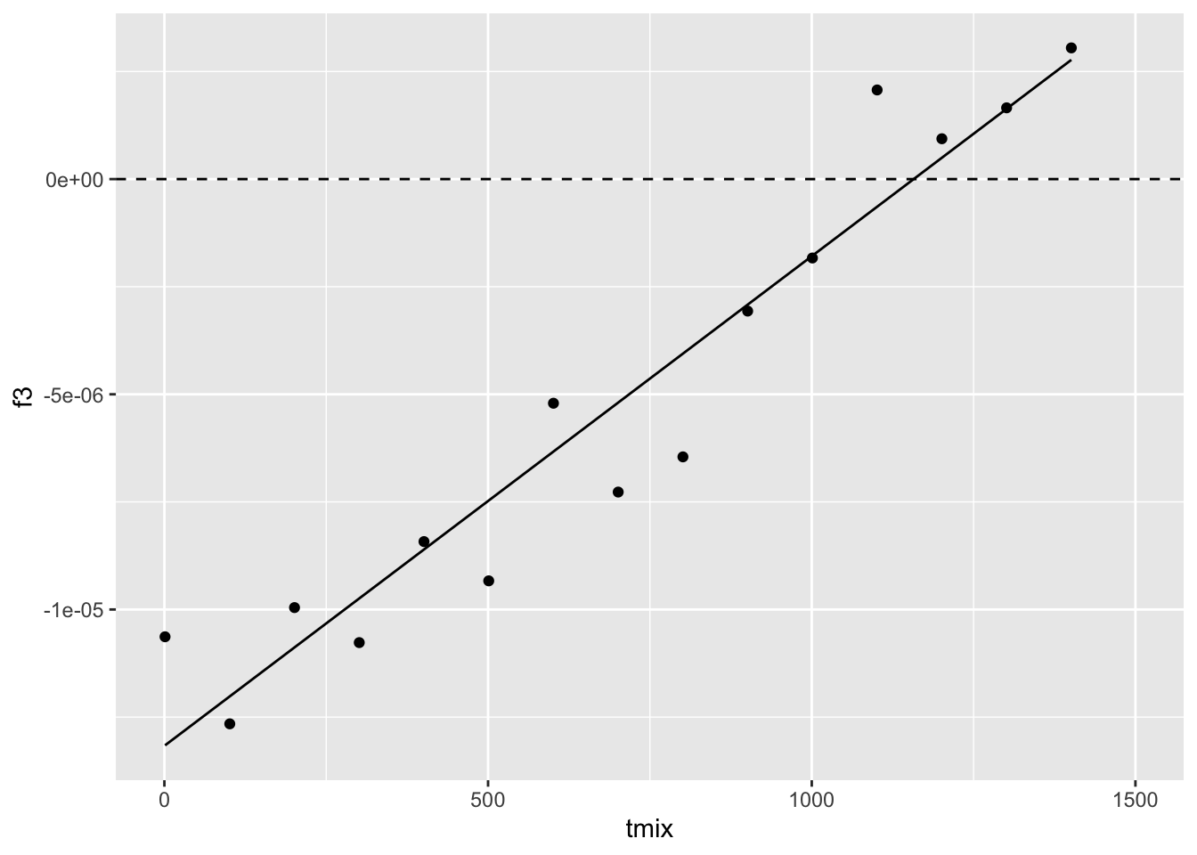
From the trend presented by the trajectory of expected \(f_3\) values as a function of the admixture time, we can see that the statistic appears to loose power to detect admixture around 1000 generations “before present” (BP).
Under which conditions would the \(f_3\) statistic gain more power?
Exercise
Fix the tadmix parameter to 1000 generations B.P. (a value at which our previous simulation suggests \(f_3\) starts losing statistical power) and Ne at 5000, and then evaluate a range of admixture proportions prop between 0% and 50% gene flow. Does \(f_3\) pick up the admixture signal for any of these admixture proportions? What does it mean for the ability of \(f_3\) to detect gene flow in our models in general?
f3_prop <- map_dfr(seq(0, 0.5, by = 0.025), compute_admix_f3, tmix = 1000, Ne = 5000)ggplot(f3_prop, aes(prop, f3)) +
geom_point() +
geom_hline(yintercept = 0, linetype = "dashed") +
geom_smooth(method = "lm", se = FALSE, color = "black", linewidth = 0.5) +
coord_cartesian(xlim = c(0, 0.5))`geom_smooth()` using formula = 'y ~ x'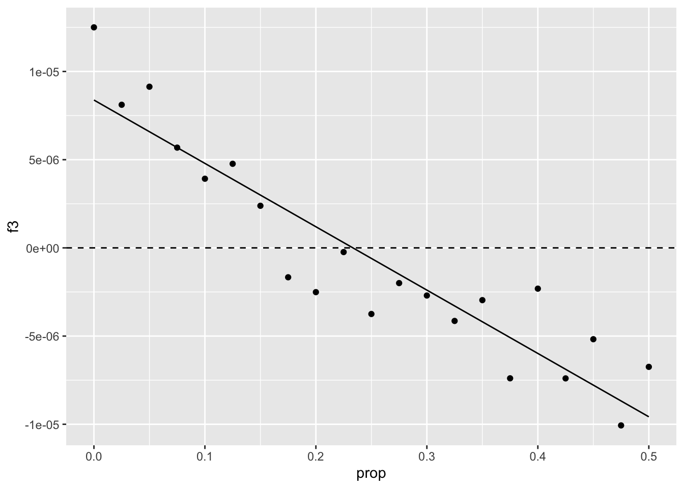
Exercise
Similarly to how you investigated the detection power of \(f_3\) as a function of admixture proportion for a given value of tmix = 1000 in the previous exercise, repeat this analysis, but now changing the Ne of the mixing population and leaving the prop parameter fixed at prop = 0.2. What do you conclude based on this analysis? Does Ne have an impact on the \(f_3\) admixture detection? If it does, why? (Look at equation XYZ.)
f3_Ne <- map_dfr(seq(1000, 20000, by = 1000), compute_admix_f3, tmix = 1000, prop = 0.2)ggplot(f3_Ne, aes(Ne, f3)) +
geom_point() +
geom_hline(yintercept = 0, linetype = "dashed") +
geom_smooth(se = FALSE, color = "black", linewidth = 0.5) +
coord_cartesian(xlim = c(1000, 20000))`geom_smooth()` using method = 'loess' and formula = 'y ~ x'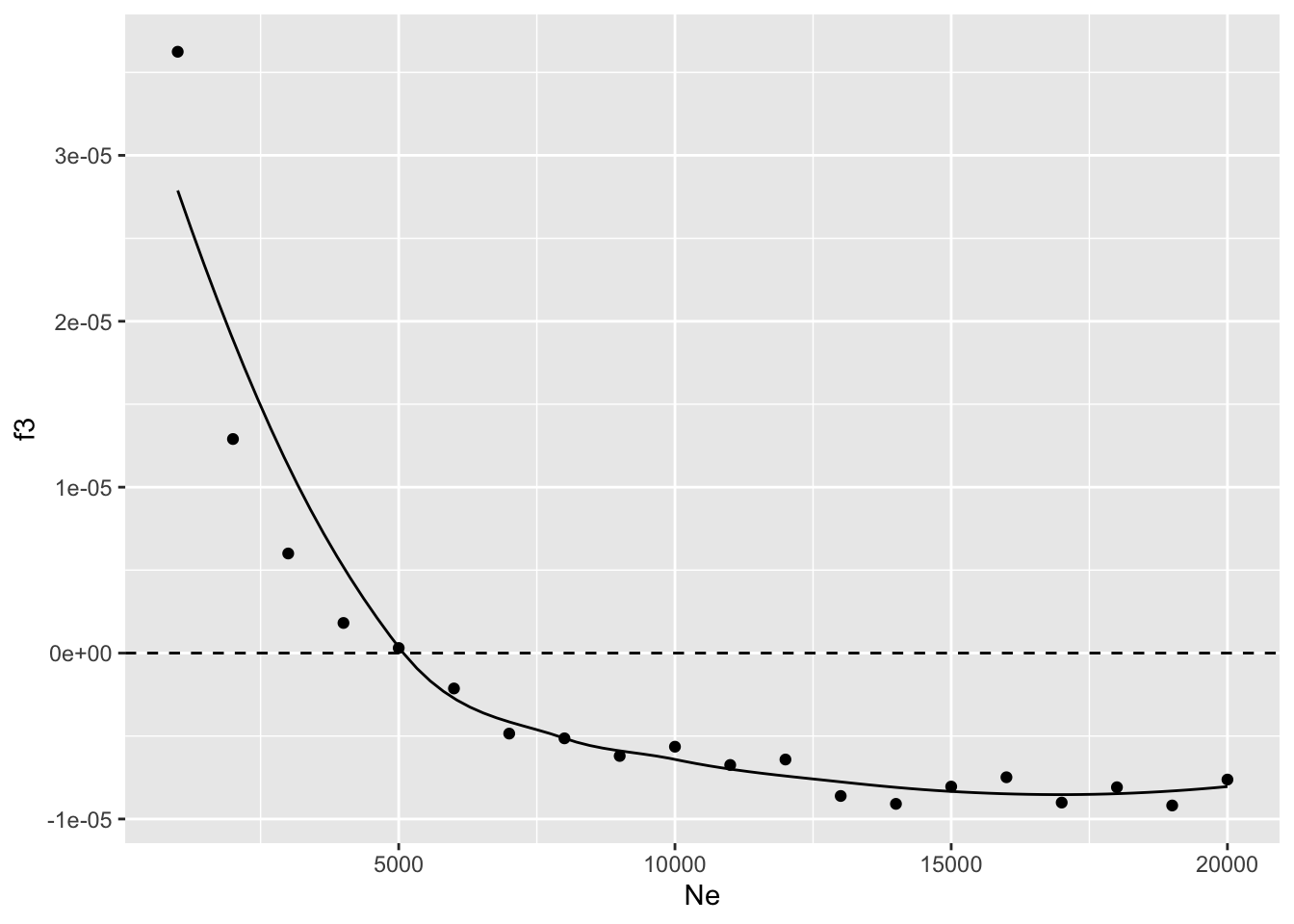
In conclusion, we can confirm that the amount of drift (represented by the Ne parameter) really is what determines whether or not can \(f_3\) detect admixture for a given model (represented by a fixed tmix time and prop admixture proportion). In fact, once we reach a certain size of the admixed population, the \(f_3\) value reaches a stable level below zero.
Exercise (extra challenge)
f3_Ne <- bind_rows(
  map_dfr(seq(1000, 20000, by = 1000), compute_admix_f3, tmix = 1000, prop = 0.1),
  map_dfr(seq(1000, 20000, by = 1000), compute_admix_f3, tmix = 1000, prop = 0.2),
  map_dfr(seq(1000, 20000, by = 1000), compute_admix_f3, tmix = 1000, prop = 0.3),
  map_dfr(seq(1000, 20000, by = 1000), compute_admix_f3, tmix = 1000, prop = 0.4),
  map_dfr(seq(1000, 20000, by = 1000), compute_admix_f3, tmix = 1000, prop = 0.5)
)ggplot(f3_Ne, aes(Ne, f3, color = factor(prop), group = factor(prop))) +
geom_point() +
geom_hline(yintercept = 0, linetype = "dashed") +
geom_smooth(se = FALSE, linewidth = 0.5) +
coord_cartesian(xlim = c(1000, 20000))`geom_smooth()` using method = 'loess' and formula = 'y ~ x'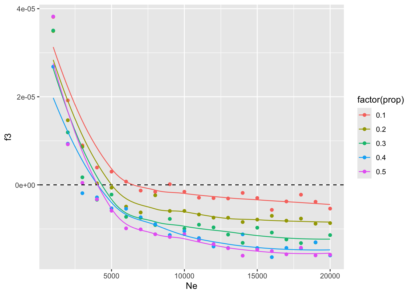
By comparing the relative position of these \(f_3\) curves with respect to the baseline null value of zero, we can see that increasing Ne of the admixed population (and, consequently, decreasing the amount of drift in that population post admixture) increases the statistical power of \(f_3\) to detect admixture even as the admixture proportion prop decreases.
Exercises
- amount of SNPs and amount of sequence vs Zscore & CI