library(dplyr)
library(tidyr)
library(readr)Basics of data science
Packages introduced in this session
Before we begin, let’s introduce the a couple of crucial parts of the tidyverse ecosystem, which we will be using extensively during exercises in this chapter.
dplyr is a centerpiece of the entire R data science universe, providing important functions for data manipulation, data summarization, and filtering of tabular data;
tidyr helps us morph untidy data into tidy data frames;
readr provides very functions for reading (and writing) tabular data. Think of it as a set of better alternatives to base R functions such as
read.table(), etc. (Another very useful package is readxl which is useful for working with Excel data).
Every single script you will be writing in this session will begin with these three lines of code.
Our example data set
Let’s also introduce a second star in this session, our example data set. The following command will read a metadata table with information about individuals published in a recent aDNA paper on the history or the Holocene in West Eurasia, dubbed “MesoNeo” (reference). Feel free to skim the paper to get an idea. If you work with anything related to human history, you’ll become closely familiar with this study.
We use the read_tsv() function (from the above-mentioned readr package) and store it in a variable df. Everything in these exercises will revolve around working with this data because it represents an excellent example of this kind of metadata table you will find across the entirety of computational population genomics. (Yes, this function is quite magical – it can read stuff from a file stored on the internet. If you’re curious about the file itself, just paste the URL address in your browser.)
df <- read_tsv("https://tinyurl.com/simgen-metadata")In addition to the brief overview from the slides for this exercise session and looking up documentation to functions via R’s ? help system, I highly encourage you to refer to this chapter of the R for Data Science text book. I keep this book at hand every time I work with R.
Create a new R script in RStudio, (File -> New file -> R Script) and save it somewhere on your computer as tidy-tables.R (File -> Save). Put the library() calls and the read_tsv() command above in this script, and let’s get started!
A selection of data-frame inspection functions
Whenever you get a new source of data, like a table from a collaborator, data sheet downloaded from supplementary materials of a paper (our situation in this session!), you need to familiarize yourself with it before you do anything else.
Here is a list of functions that you will be using constantly when doing data science to answer the following basic questions about your data.
Note: Use this list as a cheatsheet of sorts! Also, don’t forget to use the ?function command in the R console to look up the documentation to see the possibilities for options and additional features, or even just to refresh your memory. Every time I look up the ? help for a function I’ve been using for decade, I always learn new tricks.
“How many observations (rows) and variables (columns) does my data have?” –
nrow(),ncol()“What variable names (columns) am I going to be working with?” –
colnames()“What data types (numbers, strings, logicals, etc.) does it contain?” –
str(), or better,glimpse()“How can I take a quick look at a subset of the data (first/last couple of rows)?” –
head(),tail()“For a specific variable column, what is the distribution of values I can expect in that column?” –
table()for “categorical types” (types which take only a couple of discrete values),summary()for “numeric types”,min(),max(),which.min(),which.max()
Before we move on, note that when you type df into your R console, you will see a slightly different format of the output than when we worked with plain R data frames in the previous chapter. This format of data frame data is called a “tibble” and represents tidyverse’s more user friendly and modern take on data frames. For almost all practical purposes, from now on, we’ll be talking about tibbles as data frames.
Exercise 1: Exploring new data
- Inspect the
dfmetadata table using the functions above, and try to answer the following questions using the functions from the list above (you should decide which will be appropriate for which question). Before you use one of these functions for the first time, take a moment to skim through its?function_name.
How many individuals do we have metadata for?
What variables (i.e., columns) do we have in our data?
What data types (numbers, strings, logicals, etc.) are our variables of?
What are the variables we have that describe the ages (maybe look at those which have “age” in their name)? Which one would you use to get information about the ages of most individuals and why? What is the distribution of dates of aDNA individuals?
Hint: Remember that for a column/vector df$<variable>, is.na(df$<variable>) gives you TRUE for each NA element in that column variable, and sum(is.na(df$<variable>)) counts the number of NA. Alternatively, mean(is.na(df$<variable>)) counts the proportion of NA values!
How many ancient individuals do we have? How many “modern” (i.e., present-day humans) individuals?
Hint: Use the fact that for any vector (and df$groupAge is a vector, remember!), we can get the number of elements of that vector matching a certain value by applying the sum() function on a “conditional” expression, like df$groupAge == "Ancient" (which, on its own, gives TRUE / FALSE vector). In other words, in a TRUE / FALSE vector, each TRUE represents 1, and each FALSE represents 0. Obviously then, summing up such vector simply adds all the 1s together.
Who are the mysterious “Archaic” individuals? What are their names (sampleId) and which publications they come frome (dataSource)?
Hint: We need to filter our table down to rows which have groupAge == "Archaic". This is an indexing operation which you learned about in the R bootcamp session! Remember that data frames can be indexed into along two dimensions: rows and columns. You want to filter by the rows here using a logical vector obtained by df$groupAge == "Archaic".
Do we have geographical information in our metadata? Maybe countries or geographical coordinates (or even both)? Which countries do we have individuals from? (We’ll talk about spatial data science later in detail, so let’s interpret whatever geographical variable columns we have in our data frame df as any other numerical or string column variable.)
What is the source of the sequences in our data set? Does it look like they all come from a single study?
What’s the distribution of coverage of the samples? Compute the mean() and other summary() statistics on the coverage information. Why doesn’t the mean() function work when you run it on the vector of numbers in the coverage column (i.e, df$coverage, use ?mean to find the solution). Which individuals have missing coverage? Finally, use the hist() function to visualize this information to get a rough idea about the data.
These are all basic questions which you will be asking yourself every time you read a new table into R. It might not always be coverage, but you will have to do this to familiarize yourself with the data and understand its potential issues! **Always keep an eye on strange outliers, missing data NA, anything suspicious. Never take any data for granted (that applies both to data from any third parties, but even to your own data sets!).
Click to see the solution
Mean gives us NA:
mean(df$coverage)[1] NAThis is because computing the mean from a vector containing NA values is not a sensible operation – should we remove the NA values? It’s impossible to say in general, because that would depend on the nature of our data. Sometimes, encountering NA indicates a problem, so we can’t just ignore it. In situation when this is OK, there’s a argument which changes the default behavior and removes the NA elements before computing the mean:
mean(df$coverage, na.rm = TRUE)[1] 1.623767Summary takes care of the issue by reporting the number of NA values explicitly:
summary(df$coverage) Min. 1st Qu. Median Mean 3rd Qu. Max. NA's
0.0124 0.2668 0.7824 1.6238 1.5082 58.8661 2504 We can see that the coverage information is missing for 2504 individuals, which is the number of individuals in the (present-day) 1000 Genomes Project data. So it makes sense, we only have coverage for the lower-coverage aDNA samples, but for present-day individuals (who have imputed genomes), the coverage does not even make sense here.
Let’s plot the coverage values:
hist(df$coverage, breaks = 100)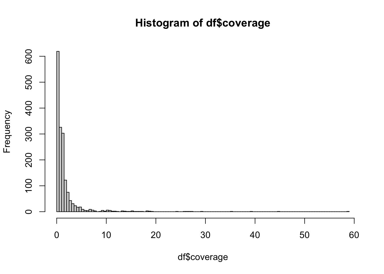
Who is the oldest individuals in our data set? Who has the highest coverage? Who has the lowest coverage?
Hint: Use functions min(), max() or which.min(), which.max(). When would you use each of the pair of functions? Look up their ?help to understand what they do and how to use them in this context.
Exercise 2: Selecting columns
Often times we end up in a situation in which we don’t want to have a large data frame with a huge number of columns. Not as much for the reasons of the data taking up too much memory, but for convenience. You can see that our df metadata table has 23 columns, which don’t fit on the screen if we just print it out (note the “13 more variables” in the output):
df# A tibble: 4,171 × 23
sampleId popId site country region groupLabel groupAge flag latitude
<chr> <chr> <chr> <chr> <chr> <chr> <chr> <chr> <dbl>
1 NA18486 YRI <NA> Nigeria WestAfrica YRI Modern 0 NA
2 NA18488 YRI <NA> Nigeria WestAfrica YRI Modern 0 NA
3 NA18489 YRI <NA> Nigeria WestAfrica YRI Modern 0 NA
4 NA18498 YRI <NA> Nigeria WestAfrica YRI Modern 0 NA
5 NA18499 YRI <NA> Nigeria WestAfrica YRI Modern 0 NA
6 NA18501 YRI <NA> Nigeria WestAfrica YRI Modern 0 NA
7 NA18502 YRI <NA> Nigeria WestAfrica YRI Modern 0 NA
8 NA18504 YRI <NA> Nigeria WestAfrica YRI Modern 0 NA
9 NA18505 YRI <NA> Nigeria WestAfrica YRI Modern 0 NA
10 NA18507 YRI <NA> Nigeria WestAfrica YRI Modern 0 NA
# ℹ 4,161 more rows
# ℹ 14 more variables: longitude <dbl>, dataSource <chr>, age14C <dbl>,
# ageHigh <dbl>, ageLow <dbl>, ageAverage <dbl>, datingSource <chr>,
# coverage <dbl>, sex <chr>, hgMT <chr>, gpAvg <dbl>, ageRaw <chr>,
# hgYMajor <chr>, hgYMinor <chr>We can select which columns to select with the function select(). It has the following general format:
select(<data frame>, <column 1>, <column 2>, ...)As a reminder, this is how we would select columns using a normal base R subsetting/indexing operation:
df[, c("sampleId", "region", "coverage", "ageAverage")]# A tibble: 4,171 × 4
sampleId region coverage ageAverage
<chr> <chr> <dbl> <dbl>
1 NA18486 WestAfrica NA NA
2 NA18488 WestAfrica NA NA
3 NA18489 WestAfrica NA NA
4 NA18498 WestAfrica NA NA
5 NA18499 WestAfrica NA NA
6 NA18501 WestAfrica NA NA
7 NA18502 WestAfrica NA NA
8 NA18504 WestAfrica NA NA
9 NA18505 WestAfrica NA NA
10 NA18507 WestAfrica NA NA
# ℹ 4,161 more rowsThis is the tidyverse approach using select():
select(df, sampleId, region, coverage, ageAverage)# A tibble: 4,171 × 4
sampleId region coverage ageAverage
<chr> <chr> <dbl> <dbl>
1 NA18486 WestAfrica NA NA
2 NA18488 WestAfrica NA NA
3 NA18489 WestAfrica NA NA
4 NA18498 WestAfrica NA NA
5 NA18499 WestAfrica NA NA
6 NA18501 WestAfrica NA NA
7 NA18502 WestAfrica NA NA
8 NA18504 WestAfrica NA NA
9 NA18505 WestAfrica NA NA
10 NA18507 WestAfrica NA NA
# ℹ 4,161 more rowsNote: The most important thing for you to note now is the absence of “double quotes”. It might not look like much, but saving yourself from having to type double quotes for every data-frame operation (like with base R) is incredibly convenient.
Practice select() by creating three new data frame objects (remember that you can assign a value to a variable using the <- operator):
- Data frame
df_ageswhich contains all variables related to sample ages - Data frame
df_geowhich contains all variables related to geography
Additionally, the first column of these data frames should always be sampleId.
Check visually (or using the ncol() functions) that you indeed have a smaller number of columns in your new data frames.
Note: select() allows us to see the contents of columns of interest much easier. For instance, in a situation in which we want to analyse the geographical location of samples, we don’t want to see columns unrelated to that – select() helps here.
If your tables has many columns of interest, typing them all by hand can become tiresome real quick. Here are a few helper functions which can be very useful in that situation:
starts_with("age")– matches columns starting with the string “age”ends_with("age")– matches columns ending with the string “age”contains("age")– matches columns containing the string “age”
Note: You can use them in place of normal column names. If we would modify our select() “template” above, we could do this, for instance:
select(<data frame object or tibble>, starts_with("text1"), ends_with("text2"))Check out the ?help belonging to those functions (note that they have ignore.case = TRUE set by default!). Then create the df_ages table again, just like earlier, with the same criteria, but use the three helper functions listed above.
Exercise 3: Filtering rows
In the chapter on base R, we learned how to filter rows using the indexing operation along the row-based dimension of (two-dimensional) data frames. For instance, in order to find out which individuals in the metadata are archaics, we first created a TRUE / FALSE vector of the rows corresponding to those individuals like this:
# get a vector of the indices belonging to archaic individuals
which_archaic <- df$groupAge == "Archaic"

# take a peek at the result to make sure we got TRUE / FALSE vector
tail(which_archaic, 10)
[1] FALSE FALSE FALSE FALSE FALSE FALSE FALSE TRUE TRUE TRUEAnd then we would use it to index into the data frame (in its first dimension, before the , comma):
archaic_df <- df[which_archaic, ]
archaic_df
# A tibble: 3 × 23
sampleId popId site country region groupLabel groupAge flag latitude
<chr> <chr> <chr> <chr> <chr> <chr> <chr> <chr> <dbl>
1 Vindija33.19 Vindi… Vind… Croatia Centr… Neanderta… Archaic 0 46.3
2 AltaiNeandertal Altai… Deni… Russia North… Neanderta… Archaic 0 51.4
3 Denisova Denis… Deni… Russia North… Denisova_… Archaic 0 51.4
# ℹ 14 more variables: longitude <dbl>, dataSource <chr>, age14C <dbl>,
# ageHigh <dbl>, ageLow <dbl>, ageAverage <dbl>, datingSource <chr>,
# coverage <dbl>, sex <chr>, hgMT <chr>, gpAvg <dbl>, ageRaw <chr>,
# hgYMajor <chr>, hgYMinor <chr>However, what if we need to filter on multiple conditions? For instance, what if we want to find only archaic individuals older than 50000 years?
One option would be to create multiple TRUE / FALSE vectors, each corresponding to one of those conditions, and then join them into a single logical vector by combining & and | logical operators like you did in the previous chapter on logical expressions. For example, we could do this:
# who is archaic in our data?
which_archaic <- df$groupAge == "Archaic"
# who is older than 50000 years?
which_old <- df$ageAverage > 50000

# who is BOTH? note the AND logical operator!
which_combined <- which_archaic & which_old
df[which_combined, ]# A tibble: 2 × 23
sampleId popId site country region groupLabel groupAge flag latitude
<chr> <chr> <chr> <chr> <chr> <chr> <chr> <chr> <dbl>
1 AltaiNeandertal Altai… Deni… Russia North… Neanderta… Archaic 0 51.4
2 Denisova Denis… Deni… Russia North… Denisova_… Archaic 0 51.4
# ℹ 14 more variables: longitude <dbl>, dataSource <chr>, age14C <dbl>,
# ageHigh <dbl>, ageLow <dbl>, ageAverage <dbl>, datingSource <chr>,
# coverage <dbl>, sex <chr>, hgMT <chr>, gpAvg <dbl>, ageRaw <chr>,
# hgYMajor <chr>, hgYMinor <chr>But this gets tiring very quickly, requires unnecessary amount of typing, and is very error prone. Imagine having to do this for many more conditions! The filter() function from tidyverse fixes all of these problems.
We can rephrase the example situation with the archaics to use the new function filter() like this:
filter(df, groupAge == "Archaic" & ageAverage > 50000)I hope that, even if you never really programmed much before, you appreciate that this single command involves very little typing and is immediately readable, almost like this English sentence:
“Filter the data frame
dffor individuals in which columngroupAgeis”Archaic” and who are older than 50000 years”.
Over time you will see that all of tidyverse packages follow these ergonomic principles.
Here is the most crucial thing for you to remember! Notice that we refer to columns of our data frame df (like the columns groupAge or ageAverage right above) as if they were normal variables! In any tidyverse function we don’t write "groupAge", but simply groupAge! When you start, you’ll probably make this kind of mistake quite often. So this is a reminder to keep an eye for this.
Practice filtering with the filter() function by finding out which individual(s) in your df metadata table are from a country with the value "CzechRepublic".
Which one of these individuals have coverage higher than 1? Which individuals have coverage higher than 10?
Exercise 4: The pipe %>%
The pipe operator, %>%, is the rockstar of the tidyverse R ecosystem, and the primary reason what makes tidy data workflow so efficient and easy to read.
First, what is “the pipe”?: whenever you see code like this:
something%>%f()
you can read it as:
“take something and put it as the first argument of f()`”.
Why would you want to do this? Imagine some complex data processing operation like this:
h(f(g(i(j(input_data)))))This means take input_data, compute j(input_data), then compute i() on that, so i(j(input_data)), then compute g(i(j(input_data))), etc. Of course this is an extreme example but is surprisingly not that far off from what we often have to do in data science.
One way to make this easier to read would be perhaps this:
tmp1 <- j(input_data)
tmp2 <- i(tmp1)
tmp3 <- g(tmp2)
tmp4 <- f(tmp3)
result <- f(tmp4)
But that’s too much typing when we want to get insights into our data as quickly as possible with as little work as possible.
The pipe approach of tidyverse would make the same thing easier to write and read like this:
input_data %>% j %>% i %>% g %>% f %>% hThis kind of “data transformation chain” is so frequent that RStudio even provides a built-in shortcut for it:
- CMD + Shift + M on macOS
- CTRL + Shift + M on Windows and Linux
Use your newly acquired select() and filter() skills, powered by the %>% piping operator, and perform the following transformation on the df metadata table (filter-ing and select-ion operations on the specified columns):
- First filter individuals for:**
- “Ancient” individuals (
groupAge) - older than 10000 years (
ageAverage) - from Italy (
country) - with
coveragehigher than 3
- Then select columns:
sampleId,site,sex, andhgMTandhgYMajor(mt and Y haplogoups).
As a practice, try to be as silly as you can and write the entire command with as many uses of filter() and select() function calls in sequence as you can.
Hint: Don’t write the entire pipeline at once, start with one condition, evaluate it, then another another one, etc., inspecting the intermediate results as you’re getting them. This is the tidyverse way of doing data science.
Hint: What I mean by this is that the following two commands produce the exact same result:
new_df1 <- filter(df, col1 == "MatchString", col2 > 10000, col3 == TRUE) %>%
  select(colX, colY, starts_with("ColNamePrefix"))
And doing this instead:
new_df1 <- df %>%
  filter(col1 == "MatchString") %>%
  filter(col2 > 10000) %>%
  filter(col3 == TRUE) %>%
  select(colX, colY, starts_with("ColNamePrefix"))
This works because “the thing on the left” (which is always a data frame) is placed by the %>% pipe operator as “the first argument of a function on the right” (which again expects always a data frame)!
Note: It is always a good practice to split long chains of %>% piping commands into multiple lines, and indenting them neatly one after the other. Readability matters to avoid bugs in your code!
Exercise 5: More complex conditions
Recall our exercises about logical conditional expression (&, |, !, etc.). You can interpret , in a filter() command as a logical &. In fact, you could also write the solution to the previous exercise:
df %>%
  filter(groupAge == "Ancient", ageAverage > 10000, country == "Italy", coverage > 1) %>%
select(sampleId, site, sex, hgMT, hgYMajor)as this:
df %>%
  filter(groupAge == "Ancient" & ageAverage > 10000 & country == "Italy" & coverage > 1) %>%
  select(sampleId, site, sex, hgMT, hgYMajor)
Whenever you need to do a more complex operation, such as saying that a variable columnX should have a value "ABC" or "ZXC", you can write filter(df, columnX == "ABC" | column == "ZXC").
Similarly, you can condition on numerical variables, just as we did in the exercises on TRUE / FALSE expressions. For instance, if you want to condition on a column varX being varX < 1 or varX > 10, you could write filter(df, varX < 1 | var X > 10).
Practice combining multiple filtering conditions into a tidyverse piping chain by filtering our metadata table to find individuals for which the following conditions hold:
- They are “Ancient” (
groupAge). - The
countryis “France” or “Canary Islands”. - Their
coverageless than 0.1 or more than 3.
Exercise 6: Dropping columns
This one will be easy. If you want to drop a column from a table, just prefix its name with a minus sign (-).
Note: Yes, this also works with starts_with() and its friends above, just put - in front of them!
Here’s our df table again (just one row for brevity):
df %>% head(1)# A tibble: 1 × 23
sampleId popId site country region groupLabel groupAge flag latitude
<chr> <chr> <chr> <chr> <chr> <chr> <chr> <chr> <dbl>
1 NA18486 YRI <NA> Nigeria WestAfrica YRI Modern 0 NA
# ℹ 14 more variables: longitude <dbl>, dataSource <chr>, age14C <dbl>,
# ageHigh <dbl>, ageLow <dbl>, ageAverage <dbl>, datingSource <chr>,
# coverage <dbl>, sex <chr>, hgMT <chr>, gpAvg <dbl>, ageRaw <chr>,
# hgYMajor <chr>, hgYMinor <chr>Observe what happens when we do this:
df %>% select(-sampleId) %>% head(1)# A tibble: 1 × 22
popId site country region groupLabel groupAge flag latitude longitude
<chr> <chr> <chr> <chr> <chr> <chr> <chr> <dbl> <dbl>
1 YRI <NA> Nigeria WestAfrica YRI Modern 0 NA NA
# ℹ 13 more variables: dataSource <chr>, age14C <dbl>, ageHigh <dbl>,
# ageLow <dbl>, ageAverage <dbl>, datingSource <chr>, coverage <dbl>,
# sex <chr>, hgMT <chr>, gpAvg <dbl>, ageRaw <chr>, hgYMajor <chr>,
# hgYMinor <chr>And this:
df %>% select(-sampleId, -site) %>% head(1)# A tibble: 1 × 21
popId country region groupLabel groupAge flag latitude longitude dataSource
<chr> <chr> <chr> <chr> <chr> <chr> <dbl> <dbl> <chr>
1 YRI Nigeria WestAfr… YRI Modern 0 NA NA 1000g
# ℹ 12 more variables: age14C <dbl>, ageHigh <dbl>, ageLow <dbl>,
# ageAverage <dbl>, datingSource <chr>, coverage <dbl>, sex <chr>,
# hgMT <chr>, gpAvg <dbl>, ageRaw <chr>, hgYMajor <chr>, hgYMinor <chr>And this:
df %>% select(-sampleId, -site, -popId) %>% head(1)# A tibble: 1 × 20
country region groupLabel groupAge flag latitude longitude dataSource age14C
<chr> <chr> <chr> <chr> <chr> <dbl> <dbl> <chr> <dbl>
1 Nigeria WestAf… YRI Modern 0 NA NA 1000g NA
# ℹ 11 more variables: ageHigh <dbl>, ageLow <dbl>, ageAverage <dbl>,
# datingSource <chr>, coverage <dbl>, sex <chr>, hgMT <chr>, gpAvg <dbl>,
# ageRaw <chr>, hgYMajor <chr>, hgYMinor <chr>The columns prefixed with - are dropped from the resulting table!
Rather than typing out a long list of columns to drop, we can also do this to specify the range of consecutive columns:
df %>% select(-(sampleId:popId)) %>% head(1)# A tibble: 1 × 21
site country region groupLabel groupAge flag latitude longitude dataSource
<chr> <chr> <chr> <chr> <chr> <chr> <dbl> <dbl> <chr>
1 <NA> Nigeria WestAfr… YRI Modern 0 NA NA 1000g
# ℹ 12 more variables: age14C <dbl>, ageHigh <dbl>, ageLow <dbl>,
# ageAverage <dbl>, datingSource <chr>, coverage <dbl>, sex <chr>,
# hgMT <chr>, gpAvg <dbl>, ageRaw <chr>, hgYMajor <chr>, hgYMinor <chr>Alternatively, we can also use our well-known c() function, which is very useful whenever we want to drop a non-consecutive set of columns:
df %>% select(-c(sampleId, site, popId)) %>% head(1)# A tibble: 1 × 20
country region groupLabel groupAge flag latitude longitude dataSource age14C
<chr> <chr> <chr> <chr> <chr> <dbl> <dbl> <chr> <dbl>
1 Nigeria WestAf… YRI Modern 0 NA NA 1000g NA
# ℹ 11 more variables: ageHigh <dbl>, ageLow <dbl>, ageAverage <dbl>,
# datingSource <chr>, coverage <dbl>, sex <chr>, hgMT <chr>, gpAvg <dbl>,
# ageRaw <chr>, hgYMajor <chr>, hgYMinor <chr>Note: The same “range syntax” of using : and and listing columns with c() applies also to selecting which columns to choose, not just for dropping them.
Use the : range in select() to drop every column after country (i.e., all the way to the last column in your table).
Exercise 7: Renaming columns
Very often you read data frames in which columns have names which are either very long, containing characters which are not allowed, or generally inconvenient. Imagine a situation, in which you refer to a particular column very often in your workflow, but it takes too much time to type it out.
After discussing select() and filter(), let’s introduce another member of the tidyverse – the function rename().
The template for using it is again very easy (again, you would replace the text in <here> with appropriate symbols):
rename(<data frame>, <new name> = <old name>)Create a new data frame df_subset by doing the following:
First
select()the columnssampleId,popId,country,groupAge,ageAverage, andcoverage.Then use the
rename()function to give them a shorter name:sampleId->sample,popId->population,groupAge->set,ageAverage->age. Leave thecountryandcoveragecolumns as they are.**
A shortcut which can be quite useful sometimes is that select() also accepts the new_name = old_name syntax of the rename() function, which allows you to both select columns (and rename some of them) all at once. Create the df_subset data frame again, but this time using just select().
When would you use one or the other?
Exercise 8: Reorganizing columns
Let’s look at another useful application of the select() function and that is reordering columns. Our df metadata table has 23 columns. When we print it out, we only see a couple of them:
head(df, 3)# A tibble: 3 × 23
sampleId popId site country region groupLabel groupAge flag latitude
<chr> <chr> <chr> <chr> <chr> <chr> <chr> <chr> <dbl>
1 NA18486 YRI <NA> Nigeria WestAfrica YRI Modern 0 NA
2 NA18488 YRI <NA> Nigeria WestAfrica YRI Modern 0 NA
3 NA18489 YRI <NA> Nigeria WestAfrica YRI Modern 0 NA
# ℹ 14 more variables: longitude <dbl>, dataSource <chr>, age14C <dbl>,
# ageHigh <dbl>, ageLow <dbl>, ageAverage <dbl>, datingSource <chr>,
# coverage <dbl>, sex <chr>, hgMT <chr>, gpAvg <dbl>, ageRaw <chr>,
# hgYMajor <chr>, hgYMinor <chr>Oftentimes when doing data analysis, we often work interactively in the console, focusing on a specific subset of columns, and need to immediately see the values of our columns of interest – how can we do this?
We already know that we can use select() to pick those columns of interest, but this removes the non-selected columns from the data frame we get. Whenever we want to retain them, we can add the call to everything(), like this:
select(<data frame>, <column 1>, <column 2>, ..., everything())Which effectively moves <column 1>, <column 2>, … to the “front” of our table, and adds everything else at the end.
Select the subset of columns you selected in the previous exercise on renaming in exactly the same way, but this time add a call to everything() at the end to keep the entire data set intact (with just columns rearranged). Save the result to df again.
Exercise 9: Sorting rows based on columns
When you need to sort the rows of a data frame based on a value of one or multiple columns, you can use the function arrange(). Again, in the spirit of the consistency across the tidyverse ecosystem, it follows exactly the same format of first giving the function a data frame to operate on, followed by a list of columns to sort by.
arrange(<data frame>, <column 1>, <column 2>, ...)Note: When you want to reverse the order of the sort, you can surround the column name in a helper function desc() (standing for “descending”).
arrange(<data frame>, desc(<column 1>), desc(<column 2>), ...)Who is the oldest individual in your data who is not an archaic individual? (Remember that you can filter() out rows corresponding to archaic individuals with the condition set != "Ancient" and then pipe the result into arrange() for sorting based on the renamed column age).
Similarly, who is the youngest ancient individual in your data in terms of its dating?
Does the same approach work for sorting text? What do you get when you try sorting based on the country column?
What do you get when you try sorting based on country and then coverage? What happens when you sort based on coverage and then country? Why is there a difference?
Does it matter what order you use filter() (on some column) and arrange() (on another column) if you’re using both functions? If yes, why? If not, why not? Think about the amount of work these functions have to do.
Exercise 10: Mutating tables
Mutating a table means adding a column for a new variable. Again, as with the previously introduced functions select(), filter(), and rename() and arrange(), it follows a consistent _tidyverse_pattern:
df %>% mutate(<new column name> = <vector of the required length>)Not surprisingly, the new column is assigned a vector of the same length as the number of rows in a data frame. What we often do is this:
df %>% mutate(<new column name> = <expression involving other columns>)because mutate() allows us to refer to other columns in the data frame already present.
To demonstrate this on a couple of exercises, let’s actually remove some columns from our data frame first. They were originally created by mutate() in the first place and this gives as a useful opportunity for practice:
df <- select(df, -set)Don’t worry, we’ll be adding them back soon using our custom code.
The important aspect of mutate is that it is a vectorized operation. We can’t create a column and give values to only some rows. Here are several ways how we could do this:
1. if_else()
if_else() accepts a logical vector (i.e., a vector of TRUE / FALSE values), and produces another vector which contains one value for each TRUE, and another value for each FALSE. Here is an example:
v <- c(TRUE, TRUE, FALSE, TRUE, FALSE)

if_else(v, 1, -1)
[1] 1 1 -1 1 -1Notice that we get 1 for each TRUE and -1 for each FALSE.
This can be a bit confusing, so spend a bit of time playing around with if_else(). For instance, create a different logical vector, and have the function produce values “hello” and “bye” depending on TRUE / FALSE state of each element. Just get familiar with this vectorized thinking because whenever we do data science, it almost always happens in this vectorized fashion (such as operating on every single value in a column of a table at once).
This function is extremely useful whenever we need to generate values of a new column based on values of another column(s). The general pattern for using it inside a mutate() call is this:
df %>%
  mutate(<new_column> = if_else(<logical vector>, true_value, false_value))
You can see that the column df$sex contains chromosome sex determination of each individual as either XY or XX. Use the if_else() function in a mutate() call to create a new column sex_desc which will contain a character vector of either “male” or “female” depending on the sex chromosome determination.
Run table(df$sex, df$sex_value) to make sure the assignment of sex description worked as expected. How do you interpret the results? Did we miss something? If we did, what is wrong?
It turns out there is an individual with a Klinefelter syndrome. A male carrying an extra X chromosome. Clearly the logic of our if_else() is incorrect because this individual was incorrectly assigned as “female”. How would you fix the mutate() command to work correctly?
Always remember to check assumptions in your data, even the ones you consider trivial. Functions such as table() and unique() are extremely useful for this.
Let’s practice if_else() a bit more. First, use filter() to look at the values of the age column for present-day individuals in the 1000 Genomes Project data (dataSource == "1000g"). What ages do you see?
You already know that you can get a logical vector indicating whether a certain element of another vector (here, the column age) is NA or not via the function is.na(). Use is.na(age) in the if_else() to set the age column with the mutate() function so that:
- Rows where
is.na(age)isTRUEare set to 0, and - Rows where
is.na(age)isFALSEare set toage(because those values don’t need to be replaced).
Note: Using mutate() to replace values of an existing column (rather than creating a new column) is done very often in data science, particularly in “clean up” operations like this one.
2. case_when()
if_else() does only work on binary TRUE or FALSE conditions. But what if we want to create a new column with values of multiple categories, not just two. Recall our original column set, which had values either “Archaic”, “Ancient”, or “Modern”.
For this purpose, case_when() is perfect. It works in a very similar manner to if_else(). Consider this vector of numbers between 1 and 30:
v <- 1:20If we wanted to assign a value “less_than_10” or “10_or_more” to each element, we could use the function if_else() like this:
if_else(v < 10, "less than 10", "10 or more") [1] "less than 10" "less than 10" "less than 10" "less than 10" "less than 10"
[6] "less than 10" "less than 10" "less than 10" "less than 10" "10 or more"
[11] "10 or more" "10 or more" "10 or more" "10 or more" "10 or more"
[16] "10 or more" "10 or more" "10 or more" "10 or more" "10 or more" What if we want to introduce three or more categories? case_when() to the rescue!
case_when(
  v < 10  ~ "less than 5",
  v == 10 ~ "exactly 10",
  v > 10 ~ "more than 10"
)
[1] "less than 5" "less than 5" "less than 5" "less than 5" "less than 5"
[6] "less than 5" "less than 5" "less than 5" "less than 5" "exactly 10"
[11] "more than 10" "more than 10" "more than 10" "more than 10" "more than 10"
[16] "more than 10" "more than 10" "more than 10" "more than 10" "more than 10"Remember how we had a slightly annoying time with doing vectorized conditional logical expressions on TRUE / FALSE vectors? Now it’s all paying off! Every one of the three conditions actually result in a logical vector, and case_when() decides which value to produced for each element of that vector based on whichever results in TRUE
The case_when() function has a very useful optional argument called .default =, which determines the value it should return whenever a particular location in the logical vector either results in all FALSE (so none of the conditions would apply), or whenever it produces a NA value (so none of the conditions can apply even in principle).
First, let’s start simple and reimplement the mutate() operation to add the sex_desc column again, this time using case_when() and implementing the three conditions (“XX”, “XY”, “XXY”) individually. Additionally, use the .default = argument of case_when() to assign “unknown” as a value of the sex_desc column.
In the exercise on conditional expressions, you learned about & and | operators which make it possible to combine multiple conditions into a single TRUE / FALSE vector. Of course, this means that the conditions inside the case_when() function can also utilize those operators.
Create a new column sex_set which will contain the following values:
sex == "XX" & age == 0" should produce“female (present-day)”`,(sex == "XY" | sex == "XXY") & age == 0" should produce“male (present-day)”`,sex == "XX" & age > 0" should produce“female (ancient)”`,(sex == "XY" | sex == "XXY") & age > 0" should produce“male (ancient)”`,- any other combination should default to “other”
I provided the logical conditions for you, you just have to put them in a case_when() call appropriately, modifying the solution to the previous exercise. Verify the outcome by doing table(df$sex_set) again.
Why did I put parenthesis around the sub-clause involving the | OR operator? What happens if we don’t do this?
Let’s ramp up the difficulty a bit more. Don’t panic! I promise things in tidyverse aren’t going to get more complicated after this, as far as your day-to-day data science work will be concerned.
First, let’s consider the region column which contains the following values:
unique(df$region) [1] "WestAfrica" "EastAfrica" "SouthernEurope"
[4] "WesternEurope" "NorthernEurope" "SouthAsia"
[7] "SouthEastAsia" "EastAsia" "NorthAmerica"
[10] "SouthAmerica" "SouthAfrica" "CentralAfrica"
[13] "NorthAfrica" "CentralEasternEurope" "WesternAsia"
[16] "CentralAsia" "NorthAsia" Here are these vectors encoded as lists, one element of the list corresponding to a continent. Copy this in your code (I premade this for you to save you some typing):
continents <- list(
  Africa = c("WestAfrica", "EastAfrica", "SouthAfrica", "CentralAfrica", "NorthAfrica"),
  Asia = c("SouthAsia", "SouthEastAsia", "EastAsia", "WesternAsia", "CentralAsia", "NorthAsia"),
  America = c("NorthAmerica", "SouthAmerica"),
  Europe = c("SouthernEurope", "WesternEurope", "NorthernEurope", "CentralEasternEurope"
)
)
Use your knowledge of the %in% operator (introduced in the R bootcamp exercise on indexing using logical vectors) and the fact that you can get an element of a named list such as continents$Africa, to create a new column called continent using the case_when() function.
Hint: As a reminder, this is how you can use the %in% operator to test whether any given element of a vector is a member of another vector (which can be used as a condition in case_when(), remember!). So, the general pattern of case_when() that you would use inside a mutate() call would be this:
case_when(
  region %in% continents$"<a continent name>") ~ "<a continent name>",
  ...
)Use the table() function on the region and continent columns of df to make sure we didn’t miss an item as we did with the sex_desc above.
Note: Always do these kinds of little sanity checks when doing transformations of your data. A little bug can always creep in and really break your analysis.
Remember how we removed the set column, which originally contained values “Modern”, “Ancient”, or “Archaic”, depending on whether the individual was a present-day modern human, ancient modern human, or an archaic individual, respectively? Use what you learned in this exercise on if_else() or case_when() to reconstruct this column again based on information in the remaining columns. (There is many possible solutions, so don’t be afraid to think creatively!)
Hint: Using information in age and the names of the three archaic individuals (combined with the .default argument of case_when() is probably the easiest solution).
Note the use of .after = in my solution to the previous exercise. Look up the help of mutate() in ?mutate to see what it does and why I used it.
Exercise 12: Summarizing tables
You have already learned how to operate on rows (filter(), arrange()), columns (select(), rename()), and both (mutate()). We have one remaining piece of the puzzle and that is operating on groups of rows. This takes the tidyverse functionality to an entire whole level and allows you to do many more powerful things with tabular data and compute summary statistics. In this section, we will will cover the functions group_by(), summarize(), and various associated “slice functions”.
1. group_by()
Take a look at the first couple of rows of our data again:
df# A tibble: 4,171 × 26
sample population country age coverage set site region groupLabel flag
<chr> <chr> <chr> <dbl> <dbl> <chr> <chr> <chr> <chr> <chr>
1 NA18486 YRI Nigeria 0 NA Mode… <NA> WestA… YRI 0
2 NA18488 YRI Nigeria 0 NA Mode… <NA> WestA… YRI 0
3 NA18489 YRI Nigeria 0 NA Mode… <NA> WestA… YRI 0
4 NA18498 YRI Nigeria 0 NA Mode… <NA> WestA… YRI 0
5 NA18499 YRI Nigeria 0 NA Mode… <NA> WestA… YRI 0
6 NA18501 YRI Nigeria 0 NA Mode… <NA> WestA… YRI 0
7 NA18502 YRI Nigeria 0 NA Mode… <NA> WestA… YRI 0
8 NA18504 YRI Nigeria 0 NA Mode… <NA> WestA… YRI 0
9 NA18505 YRI Nigeria 0 NA Mode… <NA> WestA… YRI 0
10 NA18507 YRI Nigeria 0 NA Mode… <NA> WestA… YRI 0
# ℹ 4,161 more rows
# ℹ 16 more variables: latitude <dbl>, longitude <dbl>, dataSource <chr>,
# age14C <dbl>, ageHigh <dbl>, ageLow <dbl>, datingSource <chr>, sex <chr>,
# hgMT <chr>, gpAvg <dbl>, ageRaw <chr>, hgYMajor <chr>, hgYMinor <chr>,
# sex_desc <chr>, sex_set <chr>, continent <chr>Now run the following code in your R console and carefully inspect the output (and compare it to the result of the previous command):
group_by(df, continent)# A tibble: 4,171 × 26
# Groups: continent [4]
sample population country age coverage set site region groupLabel flag
<chr> <chr> <chr> <dbl> <dbl> <chr> <chr> <chr> <chr> <chr>
1 NA18486 YRI Nigeria 0 NA Mode… <NA> WestA… YRI 0
2 NA18488 YRI Nigeria 0 NA Mode… <NA> WestA… YRI 0
3 NA18489 YRI Nigeria 0 NA Mode… <NA> WestA… YRI 0
4 NA18498 YRI Nigeria 0 NA Mode… <NA> WestA… YRI 0
5 NA18499 YRI Nigeria 0 NA Mode… <NA> WestA… YRI 0
6 NA18501 YRI Nigeria 0 NA Mode… <NA> WestA… YRI 0
7 NA18502 YRI Nigeria 0 NA Mode… <NA> WestA… YRI 0
8 NA18504 YRI Nigeria 0 NA Mode… <NA> WestA… YRI 0
9 NA18505 YRI Nigeria 0 NA Mode… <NA> WestA… YRI 0
10 NA18507 YRI Nigeria 0 NA Mode… <NA> WestA… YRI 0
# ℹ 4,161 more rows
# ℹ 16 more variables: latitude <dbl>, longitude <dbl>, dataSource <chr>,
# age14C <dbl>, ageHigh <dbl>, ageLow <dbl>, datingSource <chr>, sex <chr>,
# hgMT <chr>, gpAvg <dbl>, ageRaw <chr>, hgYMajor <chr>, hgYMinor <chr>,
# sex_desc <chr>, sex_set <chr>, continent <chr>You can probably see that the data hasn’t changed at all (same number of columns, same number of rows, all remains the same), but you can notice a new piece of information in the output:
[...]
# Groups:   continent [4]
[...]
The output says that the data has been grouped by the column/variable continent. This means that any subsequent operation will be applied not to individual rows, like it was with our mutate() operations earlier, but they will now work “per continent”. You can imagine this as the group_by() function adding a tiny bit of invisible annotation data which instructs downstream functions to work per group.
Before we move on to computing summary statistics, let’s also note that we can, of course, group based on multiple columns. For instance, in our data, we should probably not summarize based on continent but also on age, splitting individuals based on the broad age sets like this:
group_by(df, continent, set)# A tibble: 4,171 × 26
# Groups: continent, set [10]
sample population country age coverage set site region groupLabel flag
<chr> <chr> <chr> <dbl> <dbl> <chr> <chr> <chr> <chr> <chr>
1 NA18486 YRI Nigeria 0 NA Mode… <NA> WestA… YRI 0
2 NA18488 YRI Nigeria 0 NA Mode… <NA> WestA… YRI 0
3 NA18489 YRI Nigeria 0 NA Mode… <NA> WestA… YRI 0
4 NA18498 YRI Nigeria 0 NA Mode… <NA> WestA… YRI 0
5 NA18499 YRI Nigeria 0 NA Mode… <NA> WestA… YRI 0
6 NA18501 YRI Nigeria 0 NA Mode… <NA> WestA… YRI 0
7 NA18502 YRI Nigeria 0 NA Mode… <NA> WestA… YRI 0
8 NA18504 YRI Nigeria 0 NA Mode… <NA> WestA… YRI 0
9 NA18505 YRI Nigeria 0 NA Mode… <NA> WestA… YRI 0
10 NA18507 YRI Nigeria 0 NA Mode… <NA> WestA… YRI 0
# ℹ 4,161 more rows
# ℹ 16 more variables: latitude <dbl>, longitude <dbl>, dataSource <chr>,
# age14C <dbl>, ageHigh <dbl>, ageLow <dbl>, datingSource <chr>, sex <chr>,
# hgMT <chr>, gpAvg <dbl>, ageRaw <chr>, hgYMajor <chr>, hgYMinor <chr>,
# sex_desc <chr>, sex_set <chr>, continent <chr>2. summarize()
Why is grouping introduced above even useful? The most simple use case is computing summary statistics on the data on a “per group” basis using the summarize() functions. This function works a little bit like mutate(), because it creates new columns, but it only creates one row for each group.
For instance, we could compute the mean coverage of each individual in a group like this, and arrange the groups by the coverage available:
df %>%
  group_by(continent, set) %>%
  summarize(mean_coverage = mean(coverage))
`summarise()` has grouped output by 'continent'. You can override using the
`.groups` argument.# A tibble: 10 × 3
# Groups: continent [4]
continent set mean_coverage
<chr> <chr> <dbl>
1 Africa Ancient 4.99
2 Africa Modern NA
3 America Ancient 2.67
4 America Modern NA
5 Asia Ancient 1.71
6 Asia Archaic 35.3
7 Asia Modern NA
8 Europe Ancient 1.41
9 Europe Archaic 24.4
10 Europe Modern NA Notice that the result has only three columns, unlike the many columns in the original df table! We have a column for each variable we grouped over, and we have the new column with our summary statistic. Additionally, we only have 10 rows, one row for each combination of continent and set.
What does the NA value for “Modern” individuals in the output of the previous code chunk? Take a look at the original data df to answer this question.
summarize() is even more powerful than that because we can compute many different things at the same time, for each group! The next exercise is an example of that.
As you know, the mean (such as the mean_coverage we computed right above) is computed as a sum of a set of values divided by their count. Use the group_by() and summarize() code like we used above, but instead of computing the mean() directly, compute it manually by doing (in a summarize() call):
sum_coverage = sum(coverage)(the sum of coverages for each group),n = n()(the number of values in each group),mean_coverage = sum_coverage / n(using the two quantities just computed to calculate the mean)
To make things a little tidier, arrange() the results by the column mean_coverage.
Once you have your results, save this new table in a variable called df_summary.
Look up the function ?ungroup. Why is it useful?
slice_ functions
We have five “slicing” functions at our disposal, each of which extracts specific row(s) from each defined group. These functions are:
slice_head(n = 1)takes the first row,slice_tail(n = 1)takes the last row,slice_min(<column>, n = 1)takes the row with the smallest value of, slice_max(<column>, n = 1)takes the row with the largest value of, slice_sample(<col> = 1)takes one random row.
What is the lowest coverage individual in each group? While you’re doing this, filter() out the set of “Modern” individuals because they are not meaningful anyway (they have NA coverages). At the end of your %>% pipeline, pipe your results into relocate(continent, set) to make everything even tidier. Look up ?relocate to find out what this function does, if you’re not sure from the output.
Who is the oldest individual we have available on each continent?
Exercise 13: Writing (and reading) tables
Now that we have our results stored in df_summary, let’s try writing them to disk using write_tsv(). The .tsv stands for “tab-separated values” (TSV) which is a file format similar to another file you might have heard about, the “comma-separated values” (CSV) file.
Look up the help in ?write_tsv. What are the parameters you need to specify at minimum to save the file? This function has all of the useful options saved as defaults, so there’s not much you have to do. Still, look up the options!
What are other means of writing files you found in ?write_tsv? How would you read a CSV file into R? What about other file formats?
Hint: Look up ?read_csv.
Exercise 14: Some questions about the data
Which country has the highest number of aDNA samples (i.e., samples for which set == "Ancient“). How many samples from Estonia, Lithuania, or Latvia do we have?
Hint: Use the group_by(country) and summarize() combo again, together with the n() helper function.
Click to see the solution
Is there evidence of a potential bias in terms of how many samples do we have from a country and the geographical location of that country, such as the average longitude or latitude of samples from there?
Hint: Count the n count of samples from each country using group_by() and sumarize() again, like you did above, and compute also the avg_lat and avg_lon (average latitude and longitude) of samples in each country.**
Hint: Look up the linear model function ?lm or perhaps this tutorial to see how you can build a linear regression between a response variable (like our count n) and an explanatory variable (such as average longitude or latitude of a country).
countries_df <-
  df %>%
  filter(set == "Ancient") %>%
  group_by(country) %>%
  summarise(n = n(),
            avg_lat = mean(latitude, na.rm = TRUE),
            avg_lon = mean(longitude, na.rm = TRUE))

countries_df
# A tibble: 58 × 4
country n avg_lat avg_lon
<chr> <int> <dbl> <dbl>
1 Argentina 5 -50.2 -69.5
2 Armenia 6 40.1 45.3
3 Brazil 5 -19.5 -43.9
4 Cameroon 2 5.86 10.1
5 Canada 6 47.0 -94.1
6 Canary Islands 5 28.2 -16.2
7 Chile 4 -52.7 -72.9
8 China 7 43.6 93.2
9 CzechRepublic 9 49.9 15.0
10 Denmark 184 55.6 11.0
# ℹ 48 more rowsCompute the linear regression of n as a function of avg_lon – there doesn’t appear to be any significant relationship between the two variables:
lm_res <- lm(n ~ avg_lon, data = countries_df)
summary(lm_res)
Call:
lm(formula = n ~ avg_lon, data = countries_df)

Residuals:
    Min      1Q  Median      3Q     Max
-27.785 -24.543 -21.474   7.008 254.543

Coefficients:
             Estimate Std. Error t value Pr(>|t|)
(Intercept) 28.822477   7.431781   3.878 0.000279 ***
avg_lon     -0.005886   0.123753  -0.048 0.962235
---
Signif. codes:  0 '***' 0.001 '**' 0.01 '*' 0.05 '.' 0.1 ' ' 1

Residual standard error: 52.45 on 56 degrees of freedom
Multiple R-squared:  4.039e-05, Adjusted R-squared:  -0.01782
F-statistic: 0.002262 on 1 and 56 DF, p-value: 0.9622plot(countries_df$avg_lon, countries_df$n)
abline(lm_res)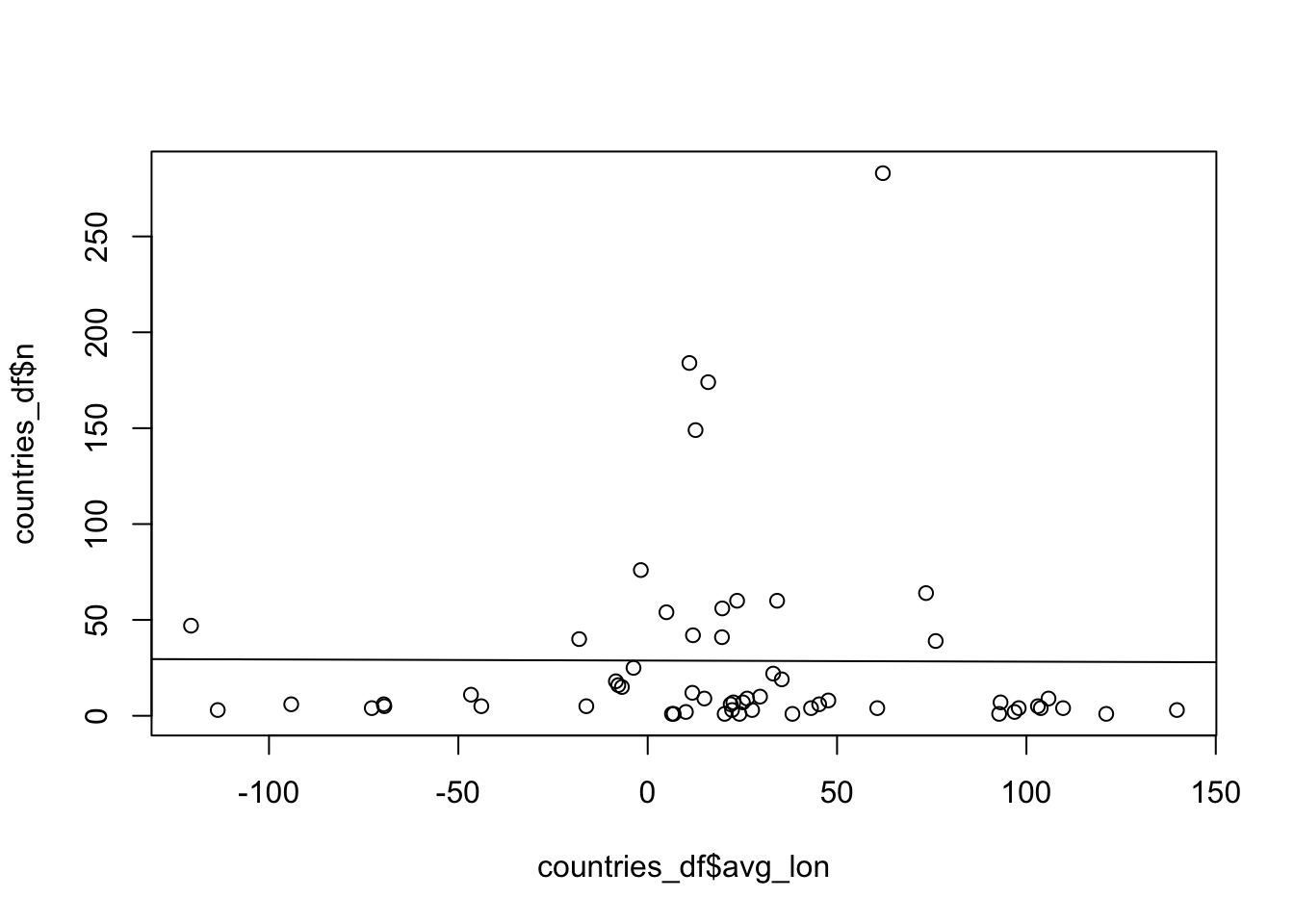
Compute the linear regression of n as a function of avg_lat – it looks like there’s a significant relationship between the number of samples from a country and geographical latitude? Is this a signal of aDNA surviving in more colder climates? :)
lm_res <- lm(n ~ avg_lat, data = countries_df)
summary(lm_res)
Call:
lm(formula = n ~ avg_lat, data = countries_df)

Residuals:
    Min      1Q  Median      3Q     Max
-41.085 -28.042 -13.834   7.972 242.851

Coefficients:
            Estimate Std. Error t value Pr(>|t|)
(Intercept)   8.2158    10.9508   0.750    0.456
avg_lat       0.5848     0.2501   2.338    0.023 *
---
Signif. codes:  0 '***' 0.001 '**' 0.01 '*' 0.05 '.' 0.1 ' ' 1

Residual standard error: 50.07 on 56 degrees of freedom
Multiple R-squared:  0.08891,   Adjusted R-squared:  0.07264
F-statistic: 5.465 on 1 and 56 DF, p-value: 0.023plot(countries_df$avg_lat, countries_df$n)
abline(lm_res)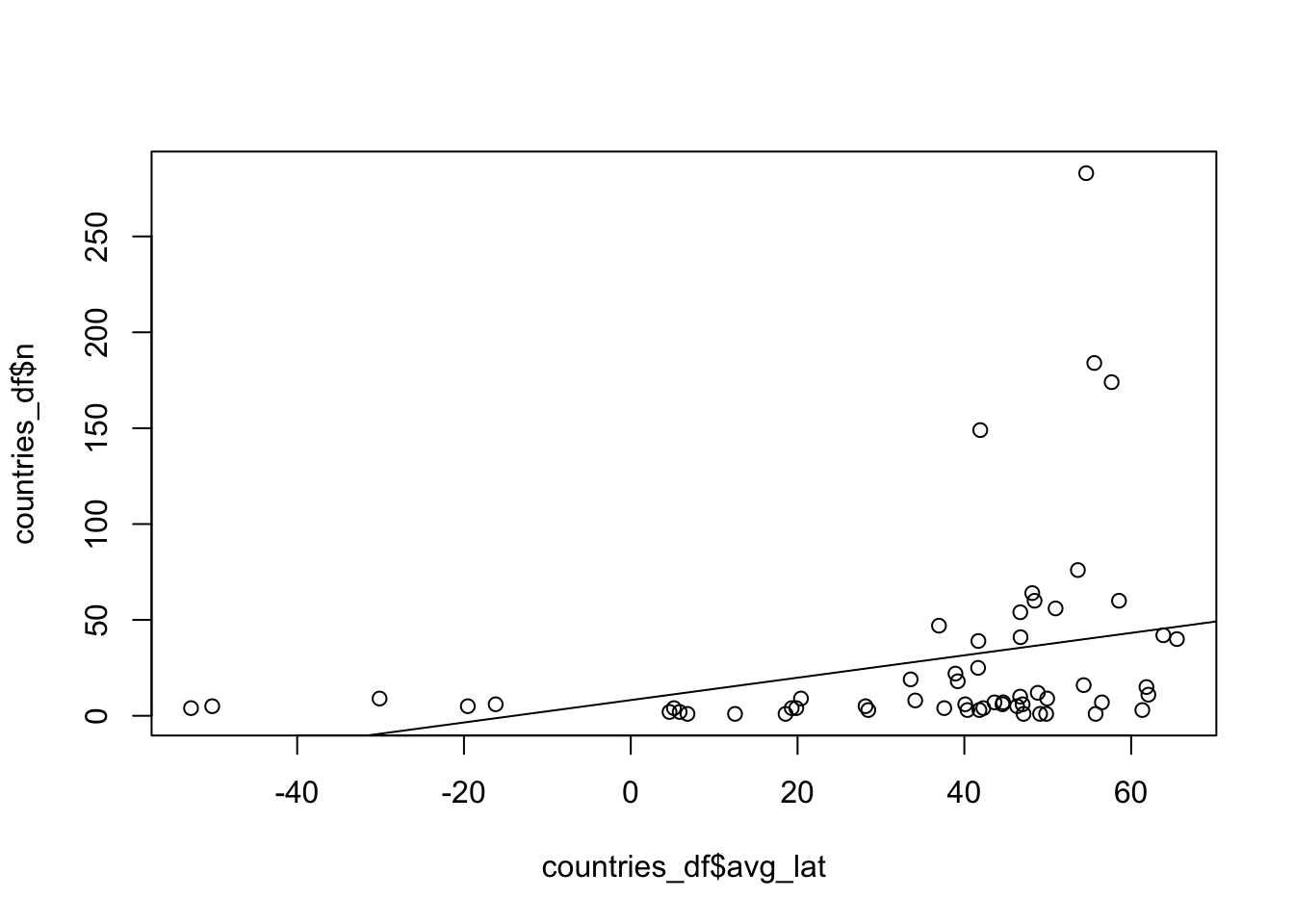
Exercise 15: tidyverse-aware functions
TODO (maybe)