⚠️⚠️⚠️
Please note that until a peer reviewed publication describing the demografr package is published, the software should be regarded as experimental and potentially unstable.
⚠️️⚠️⚠️
In order to perform probabilistic inference using a method such as Approximate Bayesian Computation, we need a way to specify prior distributions of parameters.
Different frameworks and languages approach this from different angles. This vignette describes a method used by demografr. The description provided here is quite detailed and technical. Unless you’re very curious about metaprogramming tricks provided by the R language, you’re very unlikely to need this.
Imagine the following probabilistic statements. Which features does demografr provide to encode them in an R script?
If you don’t care about technical details of demografr internals, feel free to jump here.
One trivial option
Possibly the most trivial solution to this problem in R would be to write something like the following. Indeed, some probabilistic inference R packages do exactly that:
list(
  list("Ne", "runif", 1000, 10000),
  list("geneflow", "runif", 0, 1),
  # (not sure how would one create a vector like T_i)
)
In Python, you might write object-oriented code like this:
import tensorflow_probability as tfp

# define random variables
Ne = tfp.distributions.Uniform(low=1000., high=10000.)
geneflow = tfp.distributions.Uniform(low=0., high=1.)
T_split = tfp.distributions.Uniform(low=10., high=10000.)

# sample from the distributions
Ne_sample = Ne.sample()
geneflow_sample = geneflow.sample()
T_split_sample = T_split.sample(5)
The question I asked as I began drafting the design of demografr was whether it would be possible to do this more “elegantly”—with less code and closer to actual mathematical notation.
Fancier metaprogramming solution
Despite being “a silly calculator language” (quote by a former colleague of mine), R is a very powerful functional programming language with advanced metaprogramming options. To paraphrase information from Wikipedia:
Metaprogramming is a programming technique in which computer programs have the ability to treat other programs as their data. It means that a program can be designed to read, generate, analyze or transform other programs, and even modify itself while running.
In other words, metaprogramming is when code is writing other code.
What does this mean in practice in R? You might be familiar with the syntax for fitting linear models in R:
head(mtcars)#> mpg cyl disp hp drat wt qsec vs am gear carb
#> Mazda RX4 21.0 6 160 110 3.90 2.620 16.46 0 1 4 4
#> Mazda RX4 Wag 21.0 6 160 110 3.90 2.875 17.02 0 1 4 4
#> Datsun 710 22.8 4 108 93 3.85 2.320 18.61 1 1 4 1
#> Hornet 4 Drive 21.4 6 258 110 3.08 3.215 19.44 1 0 3 1
#> Hornet Sportabout 18.7 8 360 175 3.15 3.440 17.02 0 0 3 2
#> Valiant 18.1 6 225 105 2.76 3.460 20.22 1 0 3 1
lm(cyl ~ mpg, data = mtcars)#>
#> Call:
#> lm(formula = cyl ~ mpg, data = mtcars)
#>
#> Coefficients:
#> (Intercept) mpg
#> 11.2607 -0.2525The ~ operator creates a so-called “formula
object”, which captures the expression provided by the user
(relationship between columns of the data frame, "cyl" and
"mpg"), and can then be manipulated or interpreted by the
function that the formula is passed to.
Importantly, if you type cyl ~ mpg into your R console,
you get the same thing back. It doesn’t do anything by itself! In fact,
if you were to type cyl or mpg into your R
console on their own, you would get an error.
However, when you execute the lm command above, the
function uses R’s metaprogramming features to interpret the information
in the formula to extract appropriate information (column vectors
"cyl" and "mpg") from the data frame, and
perform the necessary computation for the linear regression fit. In this
context, one could also say that the formula syntax provides a domain-specific
language for encoding statistical modeling equations in R.
Our goal in demografr, then, is to provide a similar functionality for encoding prior sampling statements.
How to use this for the problem above?
Imagine then that we want to write an R interface for doing something like this:
Obviously, we have functions such as runif,
rnorm, etc., which generate a number from a
distribution:
runif(n = 1, min = 1000, max = 10000)#> [1] 9233.254We can also do this in R, “for free”, without doing anything else.
prior <- Ne ~ runif(1000, 10000)

prior
#> Ne ~ runif(1000, 10000)Note that this expression is not evaluated! Formula is simply
an object carrying a bit of syntax. Just as we demonstrated
above in the discussion of formula used in an lm call,
simply entering Ne ~ runif(1000, 10000) into the R console
doesn’t do anything on its own.
This is important, because the runif(1000, 10000) on the
right is not a valid R code.
This is called lazy evaluation. R does not evaluate something at the time unless it’s “needed” at that time. The opposite to this is “eager evaluation” done by something like Python or C.
Metaprogramming in R in practice
Metaprogramming is often magic requiring lots of complicated tools, but to do very basic metaprogramming in R is very simple.
How can we “manipulate” code and give it our own meaning?
prior#> Ne ~ runif(1000, 10000)When given a formula, the R function as.list
parses the language expression into smallest possible “atomic
pieces”:
as.list(prior)#> [[1]]
#> `~`
#>
#> [[2]]
#> Ne
#>
#> [[3]]
#> runif(1000, 10000)This is called an abstract syntax tree in programming language design.
Note that this works generally for any language expression (even those that are much deeper):
(a + b) * (c - d / e)Although fut for expressions like the above it is easier to use a
proper metaprogramming tool such as the function ast
provided by the R package lobstr:
lobstr::ast((a + b) * (c - d / e))#> █─`*`
#> ├─█─`(`
#> │ └─█─`+`
#> │ ├─a
#> │ └─b
#> └─█─`(`
#> └─█─`-`
#> ├─c
#> └─█─`/`
#> ├─d
#> └─eEven if you haven’t heard about AST before, if you look closely at
the result above, you will notice that it captures the same expression
as (a + b) * (c - d / e) except that it dissassembled it
into smallest possible atomic pieces and decomposed it via so-called prefix
notation. This is a standard representation of AST data structure
(in fact, the simpler version we obtained via as.list above
does the same thing).
Back to demografr
Let’s now return to our original goal of encoding prior sampling statements such as :
prior#> Ne ~ runif(1000, 10000)which we can parse like this:
as.list(prior)#> [[1]]
#> `~`
#>
#> [[2]]
#> Ne
#>
#> [[3]]
#> runif(1000, 10000)And which we hope to interpret in a way that’s compatible with something like .
demografr implements a way to parse each such prior sampling statement, and automatically convert the “invalid” expression:
Ne ~ runif(1000, 10000)into a proper R statement
runif(n = 1, min = 1000, max = 10000)This is then used during the ABC simulation process.
sample_prior() function
The above feature of demografr is implemented by a function
sample_prior. Although this function is exported to the
user space in your R console, you shouldn’t need to use it for any of
your work besides simple debugging of your priors:
sample_prior(Ne ~ runif(1000, 10000))#> $variable
#> [1] "Ne"
#>
#> $value
#> [1] 9433.679
sample_prior(Ne ~ runif(1000, 10000))#> $variable
#> [1] "Ne"
#>
#> $value
#> [1] 3575.256
sample_prior(Ne ~ runif(1000, 10000))#> $variable
#> [1] "Ne"
#>
#> $value
#> [1] 8474.029This function takes in a formula statement (our DLS for encoding prior sampling events), parses it into individual components, and simulates a value of a random variable from a provided distribution function.
Sampling random vectors
To provide support for random vectors, demografr uses a similar metaprogramming trick as above.
Imagine this syntax for vectorized statements (the
T_split[5] is demografr’s made up syntax, not R
syntax!):
prior <- T_split[5] ~ runif(10, 10000)
as.list(prior)#> [[1]]
#> `~`
#>
#> [[2]]
#> T_split[5]
#>
#> [[3]]
#> runif(10, 10000)Note that this expression is one layer “deeper” than would be with a
plain T_split ~ runif(10, 10000).
This means that for “vector variables” of demografr, we need to take care of the nesting:
variable <- as.list(prior)[[2]]
variable
#> T_split[5]
as.list(variable)#> [[1]]
#> `[`
#>
#> [[2]]
#> T_split
#>
#> [[3]]
#> [1] 5In demografr then…
sample_prior(T_split[5] ~ runif(10, 10000))#> $variable
#> [1] "T_split"
#>
#> $value
#> [1] 6421.038 5195.769 7368.517 1355.319 6573.353Which internally turns the prior expression into
runif(n = 10, min = 10, max = 10000).
Final list of all priors
In conclusion, using demografr’s features it’s possible to define the example prior sampling statements from the top of this vignette in R code like this:
priors <- list(
  Ne         ~ runif(1000, 10000),
  geneflow   ~ runif(0, 1),
  T_split[5] ~ runif(10, 1000),
  truth      ~ 42
)
Take home messages:
All of this is declarative! The R code defines the priors, but doesn’t sample any numbers!
The exact process of metaprogramming that accomplishes this is something you don’t ever have to worry or care about as a user.
All of the processing and sampling from priors is done internally (and automatically) by demografr while running simulation replicates for ABC, etc., like this:
Prior parameter templates
Imagine we have the following slendr model function (hilariously overcomplicated, purely for demonstration purposes!):
library(slendr)
init_env(quiet = TRUE)

model <- function(T_a1, T_a2, T_a3, T_a4, T_a5, T_b1, T_b2, T_b3, T_b4, T_b5, N_a, N_b) {
  a1 <- population("a1", time = T_a1, N = N_a)
  a2 <- population("a2", time = T_a2, N = N_a, parent = a1)
  a3 <- population("a3", time = T_a3, N = N_a, parent = a1)
  a4 <- population("a4", time = T_a4, N = N_a, parent = a1)
  a5 <- population("a5", time = T_a5, N = N_a, parent = a1)

  b1 <- population("b1", time = T_b1, N = N_b, parent = a1)
  b2 <- population("b2", time = T_b2, N = N_b, parent = b1)
  b3 <- population("b3", time = T_b3, N = N_b, parent = b1)
  b4 <- population("b4", time = T_b4, N = N_b, parent = b1)
  b5 <- population("b5", time = T_b5, N = N_b, parent = b1)

  model <- compile_model(
    list(a1, a2, a3, a4, a5, b1, b2, b3, b4, b5),
    generation_time = 30,
  )

  return(model)
}
This functions has a huge number of parameters, so if we were to specify them with the normal DSL described above for the purposes of ABC inference, we would have to write down the following monstrosity:
individual_priors <- list(
  T_a1 ~ runif(1, 100000),
  T_a2 ~ runif(1, 100000),
  T_a3 ~ runif(1, 100000),
  T_a4 ~ runif(1, 100000),
  T_a5 ~ runif(1, 100000),
  T_b1 ~ runif(50000, 100000),
  T_b2 ~ runif(50000, 100000),
  T_b3 ~ runif(50000, 100000),
  T_b4 ~ runif(50000, 100000),
  T_b5 ~ runif(50000, 100000),

  N_a ~ runif(100, 1000),
  N_b ~ runif(200, 7000)
)
The second possibility would be to re-parametrize the function to
accept, for instance, two pairs of two vectors of T and
N, one for each population. However, we can also use
demografr’s support for ‘templated’ prior sampling
expressions (for a lack of a better word). The easiest way to
explain this is just to write it down:
templated_priors <- list(
  T_a... ~ runif(1,     100000),
  T_b... ~ runif(50000, 100000),
  N_a    ~ runif(10,    3000),
  N_b    ~ runif(1000,  10000)
)
When priors like this are plugged in to either
simulate_abc() or simulate_model(),
demografr tries to match model function arguments
against the prior names (here, T_a... and
T_b...), assigning each model function argument (i.e.,
model parameter) to an appropriate prior sampling expression by
substituting the ... on the left hand of each prior
sampling statement.
You can read T_a... ~ <distribution> as “sample
any parameter starting with ‘T_a’ from
<distribution>.
This way, when defining prior sampling expressions, you’re not hindered by the complexity of your model function (having to handle vector indexing as you’d have to with vectorized prior sampling statements).
demografr also provides means to visualize the entire prior distribution using numbers sampled from each. This can be helpful to check a previously defined prior sampling statements for correctnes:
plot_prior(individual_priors)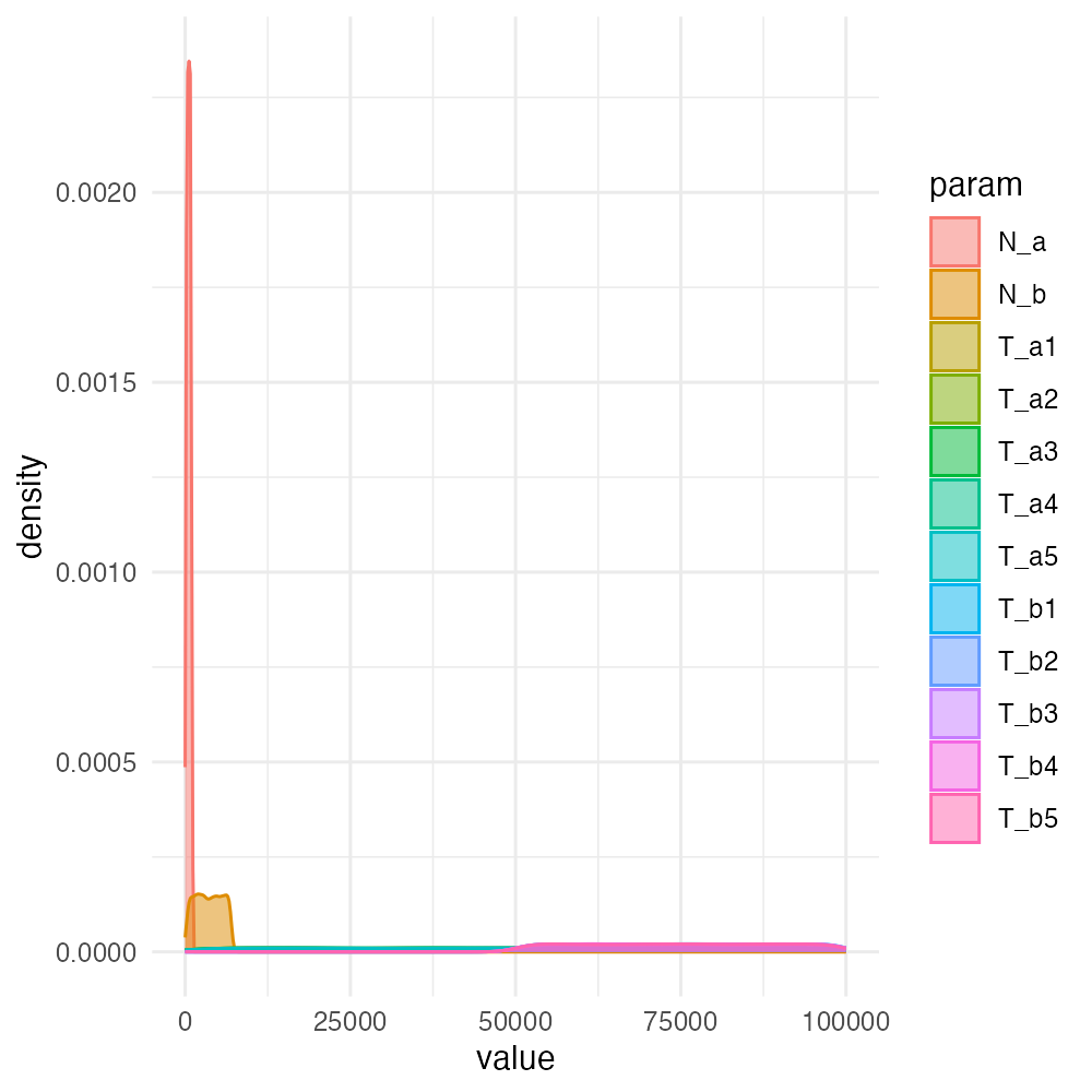
plot_prior(individual_priors, facets = TRUE)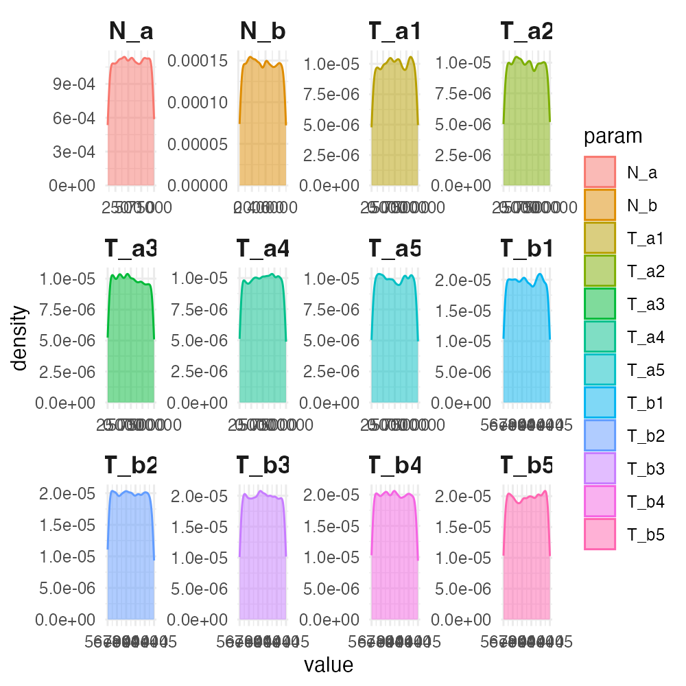
Custom functions
The DSL for specification of parameter priors also allows
custom-defined prior distribution functions, not just built-in
runif(), rnorm(), etc.
For instance, imagine this function simulating a sampling from a
distribution of a loaded casino die, rcasino():
rcasino <- function(n = 1) {
  outcomes      <- c(1, 2, 3, 4, 5, 6) # six sides of a die
  probabilities <- c(1, 1, 1, 1, 1, 3) # rolling a 6 is 3x more likely!

  sample(outcomes, size = n, prob = probabilities, replace = TRUE)
}
We can use our custom function in exactly the same way as standard R
sampling functions. First, we define a prior for sampling a parameter
value from the loaded die casino die (actually, do demonstrate that
rcasino really works as it should, let’s sample a vector of
100 random die rolls):
par <- rolls[100] ~ rcasino()During a hypothetical ABC sampling process, demografr would
then sample the parameter par (internally and
automatically) via its function sample_prior():
samples <- sample_prior(par)
samples
#> $variable
#> [1] "rolls"
#>
#> $value
#> [1] 6 5 4 6 1 4 6 6 6 6 6 6 2 5 5 5 1 6 2 4 1 6 2 6 3 5 1 6 2 6 5 1 3 4 6 1 1
#> [38] 4 1 4 3 6 6 6 3 3 4 6 6 3 4 6 3 6 1 6 5 2 6 5 2 3 6 1 2 4 6 6 3 6 6 5 6 6
#> [75] 6 5 2 4 4 6 5 2 6 6 5 6 6 6 6 2 4 3 4 4 6 6 4 1 6 2Finally, we can verify that the sampled values really correspond to a loaded die which throws a six much more often than others:
table(samples$value)#>
#> 1 2 3 4 5 6
#> 11 11 10 15 12 41