Diagnostics, model selection, troubleshooting

library(demografr)
library(slendr)
init_env()
#> The interface to all required Python modules has been activated.

library(future)
plan(multisession, workers = availableCores())

SEED <- 42
set.seed(SEED)

⚠️⚠️⚠️

The demografr R package is still under active development!

⚠️⚠️⚠️

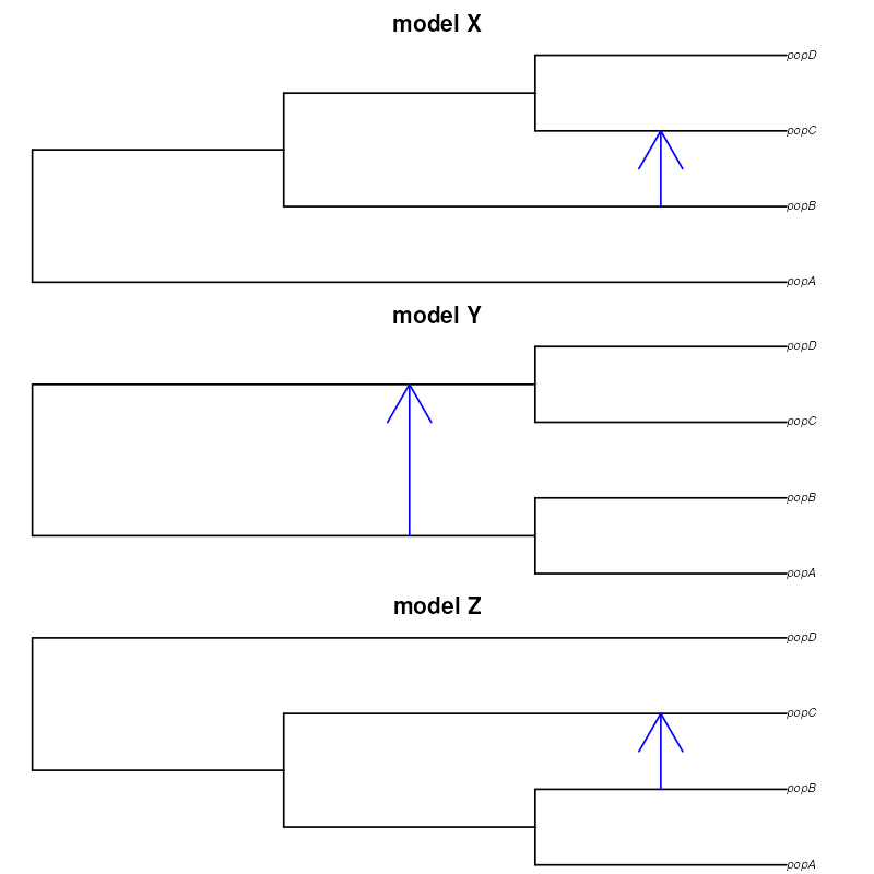
Let’s return to our first example. However, this time, imagine that we don’t really know which of the three following phylogenetic relationships is the one that captures the features of our data best, perhaps with different sources of evidence being consistent with each one of them so we want to consider all three in our modeling (as always, this is supposed to be a hypothetical example for demonstration purposes). These models differ both in terms of tree topology of the population relationships as well as in the gene flow, and we want to perform model selection.

For completeness, here is again our observed data which was, in reality, generated by a hidden evolutionary process whose parameters we’re trying to infer by doing ABC:

1. Nucleotide diversity in each population:

observed_diversity <- read.table(system.file("examples/basics_diversity.tsv", package = "demografr"), header = TRUE)

observed_diversity

#>   set    diversity
#> 1   A 8.030512e-05
#> 2   B 3.288576e-05
#> 3   C 1.013804e-04
#> 4   D 8.910909e-05

2. Pairwise divergence d_X_Y between populations X and Y:

observed_divergence <- read.table(system.file("examples/basics_divergence.tsv", package = "demografr"), header = TRUE)

observed_divergence

#>   x y   divergence
#> 1 A B 0.0002378613
#> 2 A C 0.0002375761
#> 3 A D 0.0002379385
#> 4 B C 0.0001088217
#> 5 B D 0.0001157056
#> 6 C D 0.0001100633

3. Value of the following $f_4$-statistic:

observed_f4  <- read.table(system.file("examples/basics_f4.tsv", package = "demografr"), header = TRUE)

observed_f4

#>   W X Y Z            f4
#> 1 A B C D -3.262146e-06

We will again bind them into a list:

observed <- list(
  diversity  = observed_diversity,
  divergence = observed_divergence,
  f4 = observed_f4
)

Three competing models

First, in order to perform model selection, we need to specify models themselves. We do this by defining three separate slendr functions, each of them encoding the three population relationships from the diagrams above. Note that we’re not trying to infer the time of gene flow, for simplicity, but we do fix the gene flow event to different times (again, reflected in the alternative model sketches above), just to make the models stand out from one another:

modelX <- function(Ne_A, Ne_B, Ne_C, Ne_D, T_1, T_2, T_3, gf) {
  A <- population("A", time = 1,   N = Ne_A)
  B <- population("B", time = T_1, N = Ne_B, parent = A)
  C <- population("C", time = T_2, N = Ne_C, parent = B)
  D <- population("D", time = T_3, N = Ne_D, parent = C)

  gf <- gene_flow(from = B, to = C, start = 9000, end = 9301, rate = gf)

  model <- compile_model(
    populations = list(A, B, C, D), gene_flow = gf,
    generation_time = 1, simulation_length = 10000,
    direction = "forward"
  )

  samples <- schedule_sampling(
    model, times = 10000,
    list(A, 50), list(B, 50), list(C, 50), list(D, 50),
    strict = TRUE
  )

  return(list(model, samples))
}

modelY <- function(Ne_A, Ne_B, Ne_C, Ne_D, T_1, T_2, T_3, gf) {
  A <- population("A", time = 1,   N = Ne_A)
  B <- population("B", time = T_1, N = Ne_B, parent = A)
  C <- population("C", time = T_2, N = Ne_C, parent = A)
  D <- population("D", time = T_3, N = Ne_D, parent = A)

  gf <- gene_flow(from = A, to = B, start = 9000, end = 9301, rate = gf)

  model <- compile_model(
    populations = list(A, B, C, D), gene_flow = gf,
    generation_time = 1, simulation_length = 10000,
    direction = "forward"
  )

  samples <- schedule_sampling(
    model, times = 10000,
    list(A, 50), list(B, 50), list(C, 50), list(D, 50),
    strict = TRUE
  )

  return(list(model, samples))
}

modelZ <- function(Ne_A, Ne_B, Ne_C, Ne_D, T_1, T_2, T_3, gf) {
  A <- population("A", time = 1,   N = Ne_A)
  B <- population("B", time = T_1, N = Ne_B, parent = A)
  C <- population("C", time = T_2, N = Ne_C, parent = A)
  D <- population("D", time = T_3, N = Ne_D, parent = C)

  gf <- gene_flow(from = C, to = D, start = 9000, end = 9301, rate = gf)

  model <- compile_model(
    populations = list(A, B, C, D), gene_flow = gf,
    generation_time = 1, simulation_length = 10000,
    direction = "forward"
  )

  samples <- schedule_sampling(
    model, times = 10000,
    list(A, 50), list(B, 50), list(C, 50), list(D, 50),
    strict = TRUE
  )

  return(list(model, samples))
}

Now, let’s specify priors using demografr’s templating syntax. This saves us a bit of typing, making the prior definition code a bit more consise and easier to read:

priors <- list(
  Ne... ~ runif(100, 10000),

  T_1   ~ runif(1,    4000),
  T_2   ~ runif(3000, 9000),
  T_3   ~ runif(5000, 10000),

  gf    ~ runif(0, 1)
)

Let’s also put together a list of tree-sequence summary functions and observed summary statistics:

compute_diversity <- function(ts) {
  samples <- ts_names(ts, split = "pop")
  ts_diversity(ts, sample_sets = samples)
}

compute_divergence <- function(ts) {
  samples <- ts_names(ts, split = "pop")
  ts_divergence(ts, sample_sets = samples)
}

compute_f4 <- function(ts) {
  samples <- ts_names(ts, split = "pop")
  A <- samples["A"]; B <- samples["B"]
  C <- samples["C"]; D <- samples["D"]
  ts_f4(ts, A, B, C, D)
}

functions <- list(
  diversity = compute_diversity,
  divergence = compute_divergence,
  f4 = compute_f4
)

Let’s validate the ABC setup of all three models – this is an important check that the slendr model functions are defined correctly (we set quiet = TRUE to surpress writing out the full log output):

validate_abc(modelX, priors, functions, observed, quiet = TRUE,
             sequence_length = 1e6, recombination_rate = 1e-8)
validate_abc(modelY, priors, functions, observed, quiet = TRUE,
             sequence_length = 1e6, recombination_rate = 1e-8)
validate_abc(modelZ, priors, functions, observed, quiet = TRUE,
             sequence_length = 1e6, recombination_rate = 1e-8)

With that out of the way, we can proceed with generating simulated data for inference using all three models. What we’ll do is perform three runs and save them into appropriately named variables dataX, dataY, and dataZ:

dataX <- simulate_abc(modelX, priors, functions, observed, iterations = 10000,
                      sequence_length = 10e6, recombination_rate = 1e-8, mutation_rate = 1e-8)

dataY <- simulate_abc(modelY, priors, functions, observed, iterations = 10000,
                      sequence_length = 10e6, recombination_rate = 1e-8, mutation_rate = 1e-8)

dataZ <- simulate_abc(modelZ, priors, functions, observed, iterations = 10000,
                      sequence_length = 10e6, recombination_rate = 1e-8, mutation_rate = 1e-8)

The total runtime for the ABC simulations was 1 hours 37 minutes 46 seconds parallelized across 96 CPUs.

abcX <- run_abc(dataX, engine = "abc", tol = 0.01, method = "neuralnet")
abcY <- run_abc(dataY, engine = "abc", tol = 0.01, method = "neuralnet")
abcZ <- run_abc(dataZ, engine = "abc", tol = 0.01, method = "neuralnet")

Cross-validation

Before doing model selection, it’s important to perform cross-validation to answer the question whether our ABC setup can even distinguish between the competing models. Without having the power to do this, trying to select the best model wouldn’t make much sense.

This can be done using demografr’s cross_validate() function which is built around abc’s own function cv4postpr(). We will not go into too much detail, as this function simply calls cv4postpr() under the hood, passing to it all specified function arguments on behalf of a user to avoid unnecessary manual data munging (creating the index vector, merging the summary statistics into sumstat parameter, etc.). For more details, read section “Model selection” in the vignette of the abc R package.

The one difference between the two functions is that cross_validate() removes the need to prepare character indices and bind together summary statistic matrices from different models—given that demografr’s ABC output objects track all this information along in their internals, this is redundant, and you can perform cross-validation of different ABC models simply by calling this:

models <- list(abcX, abcY, abcZ)

cv_selection <- cross_validate(models, nval = 100, tol = 0.01, method = "neuralnet")

If we print out the result, we get a quick summary of the resulting confusion matrices and other diagnostic information:

cv_selection

#> Confusion matrix based on 100 samples for each model.
#> 
#> $tol0.01
#>        modelX modelY modelZ
#> modelX     95      0      5
#> modelY      0     98      2
#> modelZ      0      1     99
#> 
#> 
#> Mean model posterior probabilities (neuralnet)
#> 
#> $tol0.01
#>        modelX modelY modelZ
#> modelX 0.8878 0.0597 0.0525
#> modelY 0.0467 0.9336 0.0197
#> modelZ 0.0097 0.0237 0.9667
#> 
#> $conf.matrix
#> $conf.matrix$tol0.01
#>        modelX modelY modelZ
#> modelX     95      0      5
#> modelY      0     98      2
#> modelZ      0      1     99
#> 
#> 
#> $probs
#> $probs$tol0.01
#>            modelX     modelY     modelZ
#> modelX 0.88777233 0.05968226 0.05254541
#> modelY 0.04670368 0.93357416 0.01972216
#> modelZ 0.00966135 0.02366910 0.96666955

Similarly, you can use the plot() function to visualize the result. This function, yet again, internally calls abc’s own plotting method internall, with a bonus option to save a figure to a PDF right from the plot() call (useful when working on a remote server):

plot(cv_selection)

Because we have three models, each of the three barplots shows how often were summary statistics sampled from each model classified as likely coming from one of the three models. In other words, with absolutely perfect classification, each barplot would show just one of the three colors. If a barplot (results for one model) shows multiple colors, this means that some fraction of simulated statistics from that model was incorrectly classified as another model. Again, for more detail on interpretation, caveats, and best practices, please consult the abc R package vignette and a relevant statistical textbook.

The confusion matrices and the visualization all suggest that ABC can distinguish between the three models very well. For instance, modelX has been classified correctly in:

cv_selection$estim[[1]] %>% { .[names(.) == "modelX"] } %>% { names(.) == . } %>% sum

#> [1] 95

simulations out of the total of 100 cross-validation simulations, with an overall misclassification rate for all models of only:

#> [1] "2.7%"

Model selection

Armed with confidence in the ability of ABC to correctly identify the correct model based on simulated data, we can proceed to selection of the best model for our empirical data set. This can be done with the function select_model() which is demografr’s convenience wrapper around abc’s own function postpr:

models <- list(abcX, abcY, abcZ)

modsel <- select_model(models, tol = 0.03, method = "neuralnet")

We can make a decision on the model selection by inspecting the summary() of the produced result:

modsel

#> Call: 
#> abc::postpr(target = parts$target, index = parts$index, sumstat = parts$sumstat, 
#>     tol = tol, method = "neuralnet")
#> Data:
#>  postpr.out$values (900 posterior samples)
#> Models a priori:
#>  modelX, modelY, modelZ
#> Models a posteriori:
#>  modelX, modelY, modelZ
#> 
#> Proportion of accepted simulations (rejection):
#> modelX modelY modelZ 
#> 0.8711 0.0056 0.1233 
#> 
#> Bayes factors:
#>          modelX   modelY   modelZ
#> modelX   1.0000 156.8000   7.0631
#> modelY   0.0064   1.0000   0.0450
#> modelZ   0.1416  22.2000   1.0000
#> 
#> 
#> Posterior model probabilities (neuralnet):
#> modelX modelY modelZ 
#>      1      0      0 
#> 
#> Bayes factors:
#>             modelX      modelY      modelZ
#> modelX      1.0000 332871.6946 524021.4981
#> modelY      0.0000      1.0000      1.5742
#> modelZ      0.0000      0.6352      1.0000

As we can see, modelX shows the highest rate of acceptance among all simulations. Specifically, we see that the proportion of acceptance is:

sprintf("%.1f%%", max(quiet(summary(modsel))$rejection$Prob) * 100)

#> [1] "87.1%"

Similarly, looking at the Bayes factors, we see that the “modelX” is

sprintf("%.1f", quiet(summary(modsel))$rejection$Bayes[1, 2])

#> [1] "156.8"

times more likely than “modelY”, and

sprintf("%.1f", quiet(summary(modsel))$rejection$Bayes[1, 3])

#> [1] "7.1"

times more likely than “modelZ”.

When the posterior probabilities are computed using a more elaborate neural network method (again, see more details in the abc vignette), we find that the probability of “modelX” is even more overwhelming. In fact, the analysis shows that it has a 100% probabiliy of being the correct model to explain our data.

But how accurate are these conclusions? Well, if we take a peek at the slendr model which was internally used to generate the “observed” summary statistics, we see that the data was indeed simulated by code nearly identical to the one shown above as modelX. When plotted, the true model looks like this:

A <- population("A", time = 1, N = 2000)
B <- population("B", time = 2000, N = 800, parent = A)
C <- population("C", time = 6000, N = 9000, parent = B)
D <- population("D", time = 8000, N = 4000, parent = C)

gf <- gene_flow(from = B, to = C, start = 9000, end = 9301, rate = 0.1)

example_model <- compile_model(
  populations = list(A, B, C, D), gene_flow = gf,
  generation_time = 1,
  simulation_length = 10000
)

plot_model(example_model, proportions = TRUE)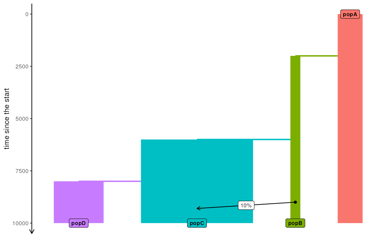

It appears that we can be quite confident in which of the three models is most compatible with the data. However, before we move on to inferring parameters of the model, we should check whether the best selected model can indeed capture the most important features of the data, which is in case of ABC represented by our summary statistics.

In order to do this, demografr provides a function call predict() which performs posterior predictive check. Below, we we also look at how to use functions gfit() and gfitpca() implemented by the abc R package itself.

Let’s start with the posterior predictive checks.

Posterior predictive checks

Link: http://www.stat.columbia.edu/~gelman/research/published/A6n41.pdf

It is one thing to Simply speaking, when fitting a model and estimating its parameters using ABC, we rely on a set of summary statistics, which we assume capture the most important features of the true model represented by the data we gathered. Performing posterior predictive checks involves estimating the posterior distributions of the parameters of interest from the data (i.e. doing ABC inference) – something we’ve done above on our modelX, modelY, and modelZ – and then sampling parameters from these distributions and generating distributions of simulated summary statistics from those estimated models. Then, we plot the distributions of each of our simulated summary statistics together with a vertical line representing the values of the observed statistics. Naturally, only if the model can generate statistics compatible with the values observed in real data can we regard the model as sensible and usable for inference.

plan(multisession, workers = availableCores())
predX <- predict(abcX, samples = 1000, posterior = "unadj")
predY <- predict(abcY, samples = 1000, posterior = "unadj")
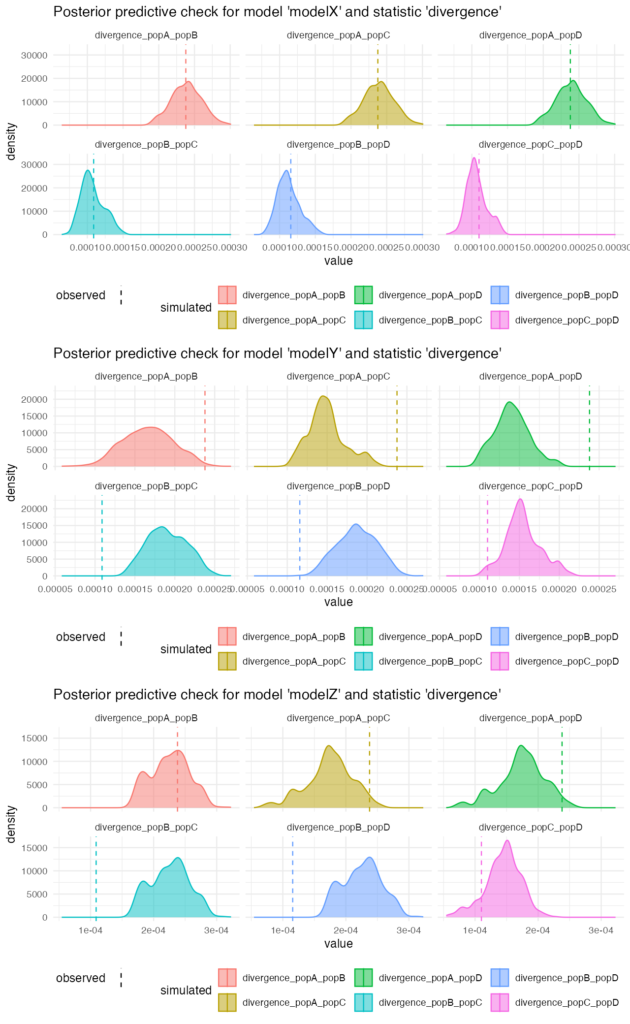
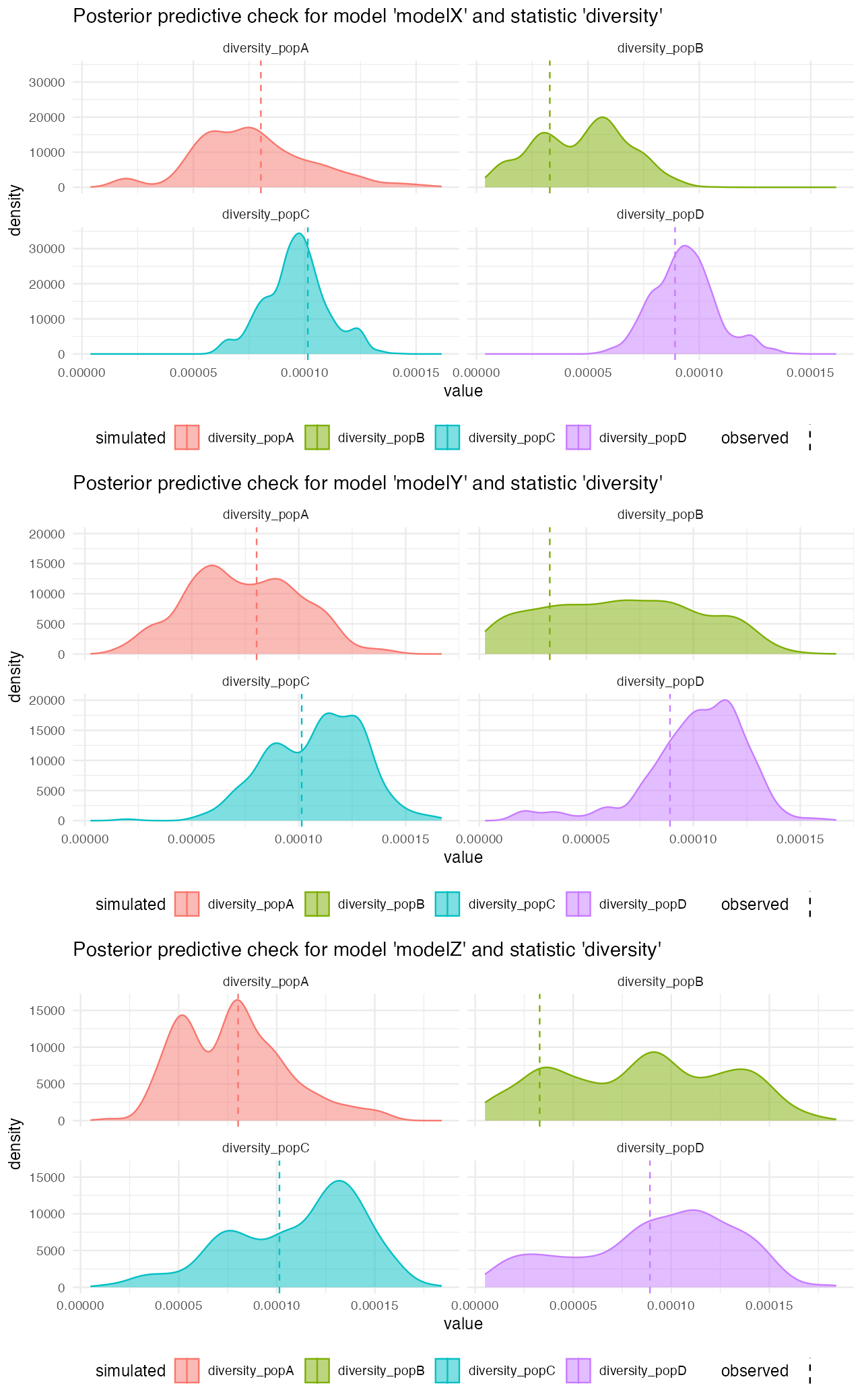
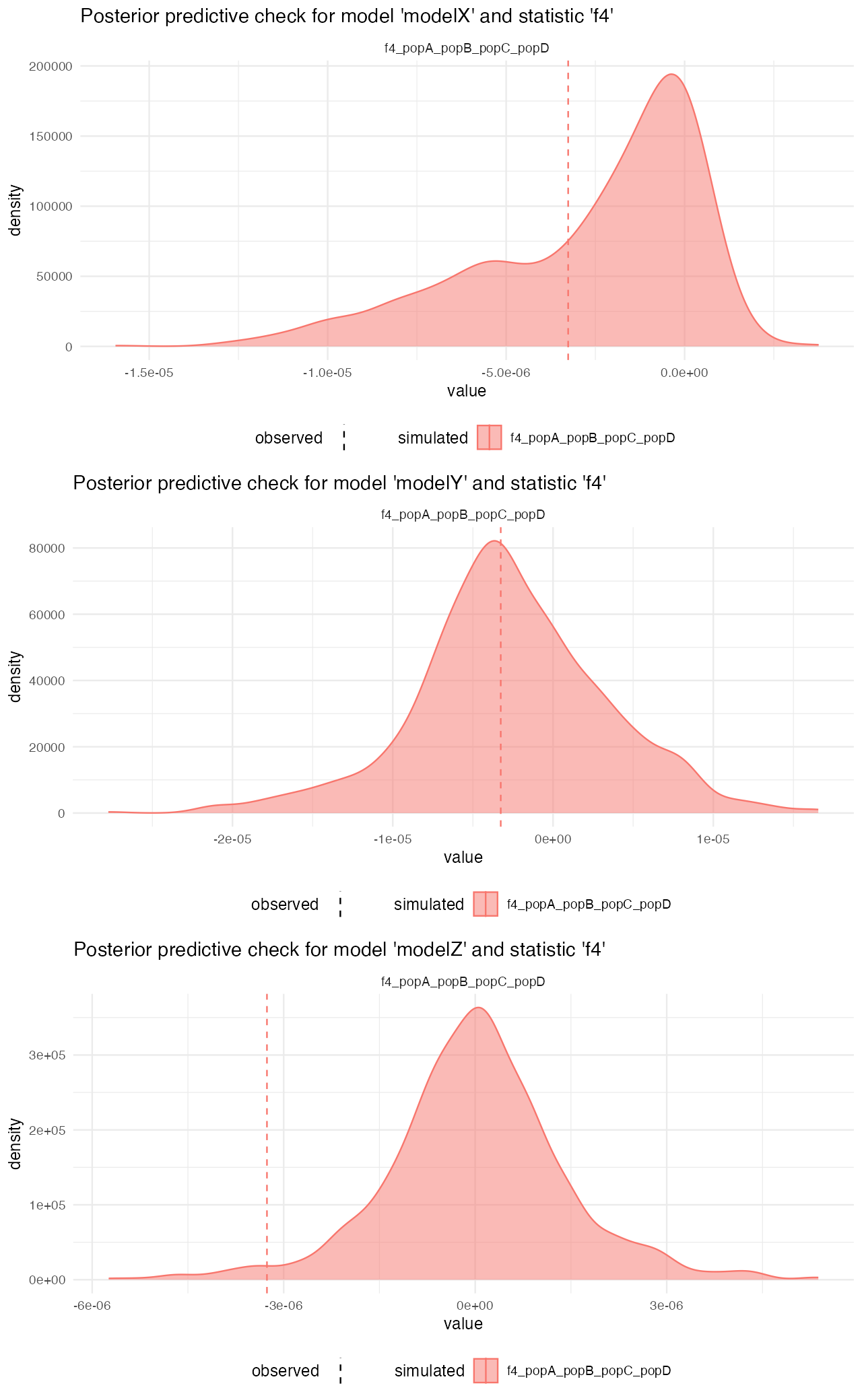
predZ <- predict(abcZ, samples = 1000, posterior = "unadj")

Looking at the posterior predictive plots from the model X, we can see that the observed statistics (vertical dashed lines) fall very well within the distributions of statistics simulated from the posterior parameters of the model. This suggests that are model (simplified that it must be given the more complex reality), captures the empoirical statistics quite well:

plot_prediction(predX)

#> $diversity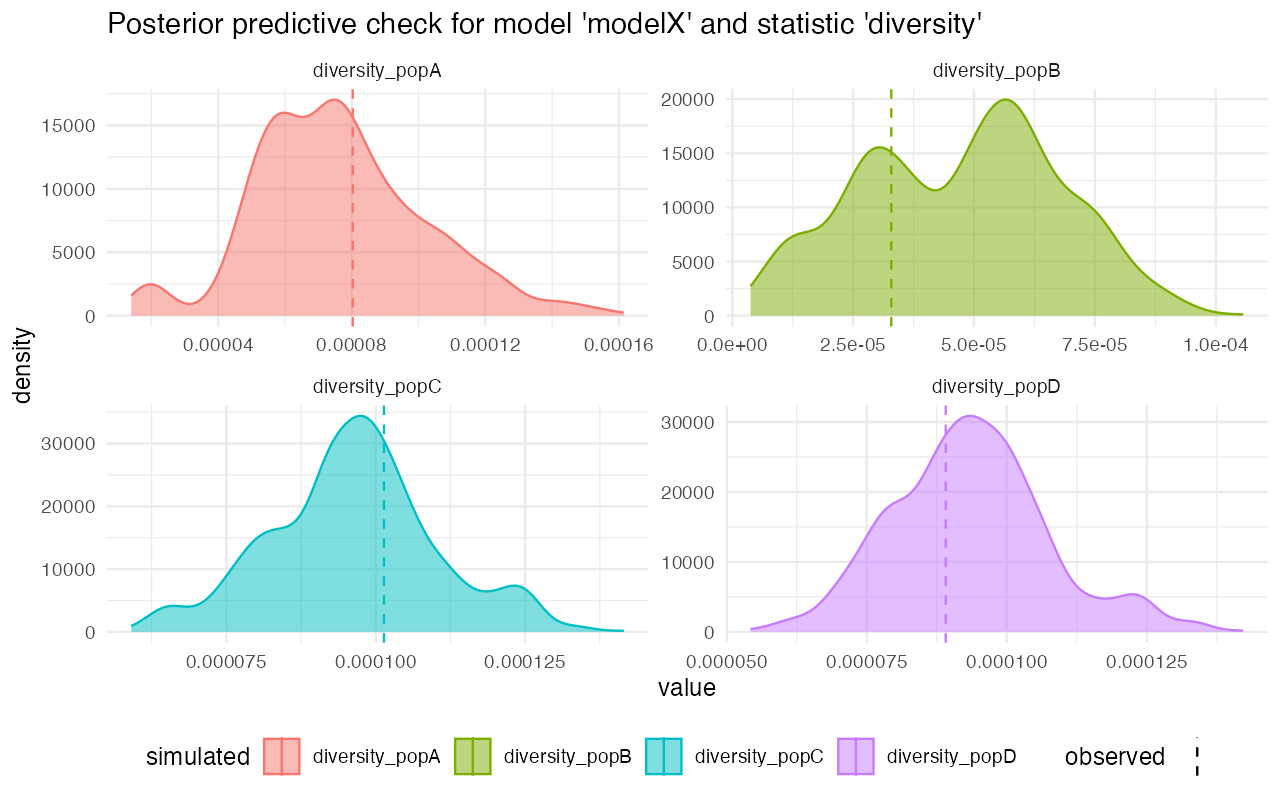

#> 
#> $divergence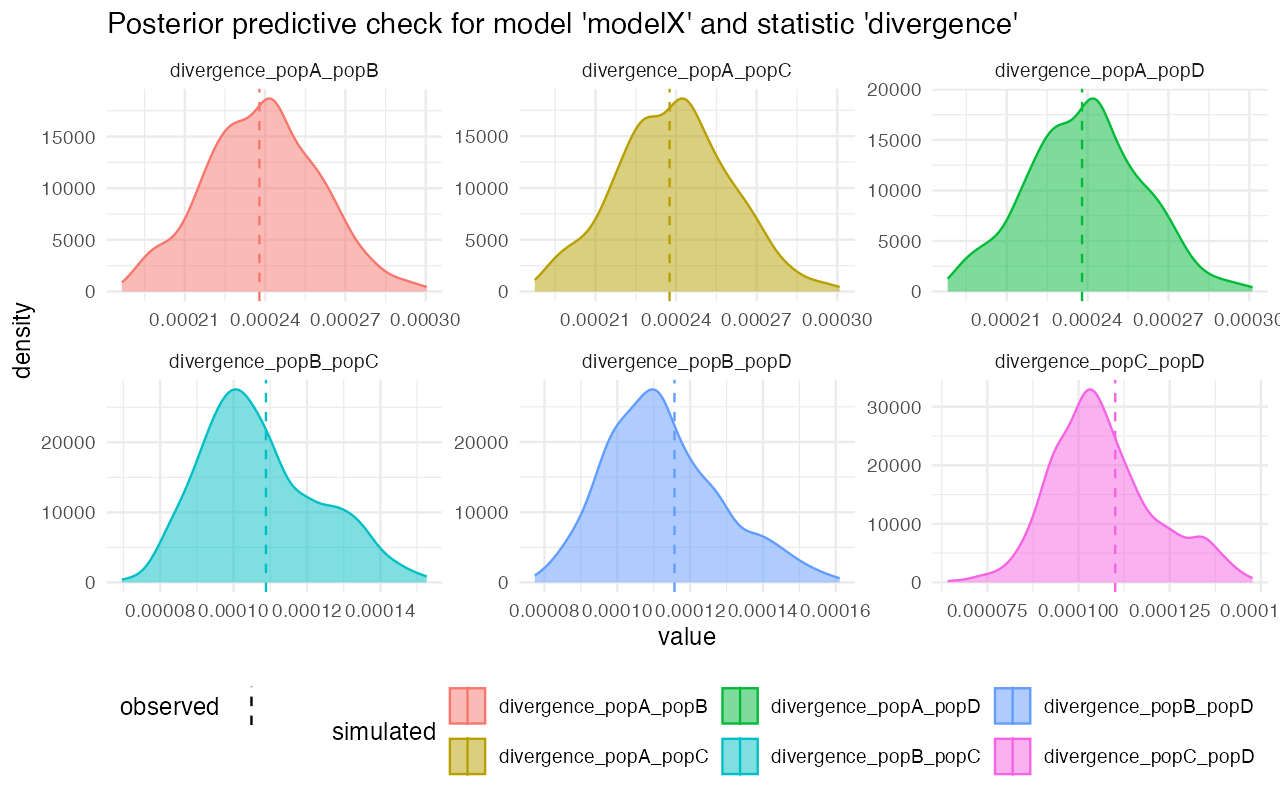

#> 
#> $f4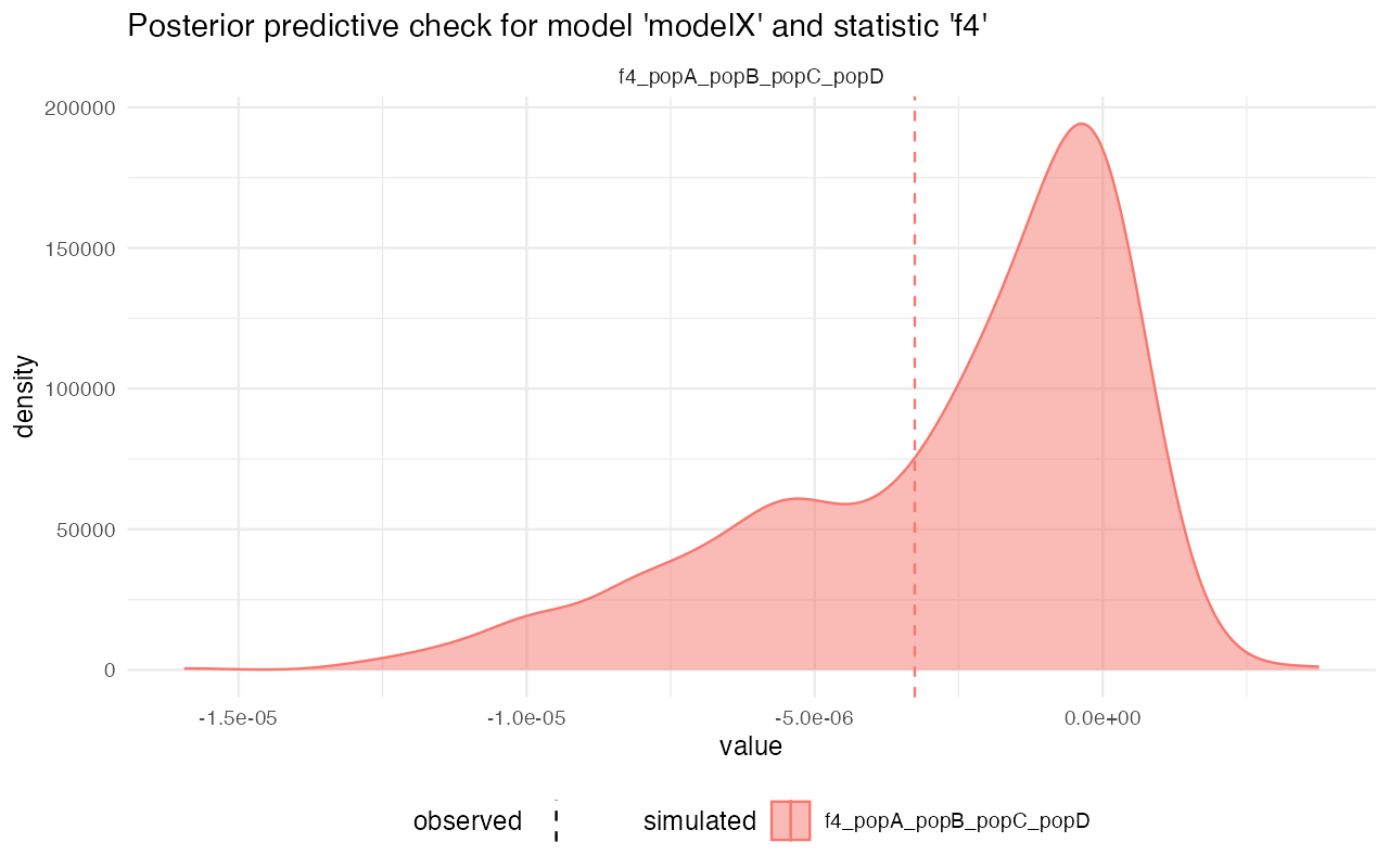

On the other hand, looking at the model Z, for instance, we see that although the $f_4$ gene-flow detection statistic fits rather nicely, the pairwise divergences between populations are completely from the statistics simulated from posterior distributions. This strongly suggests that the model wasn’t able to capture the features of the data.

plot_prediction(predY)

#> $diversity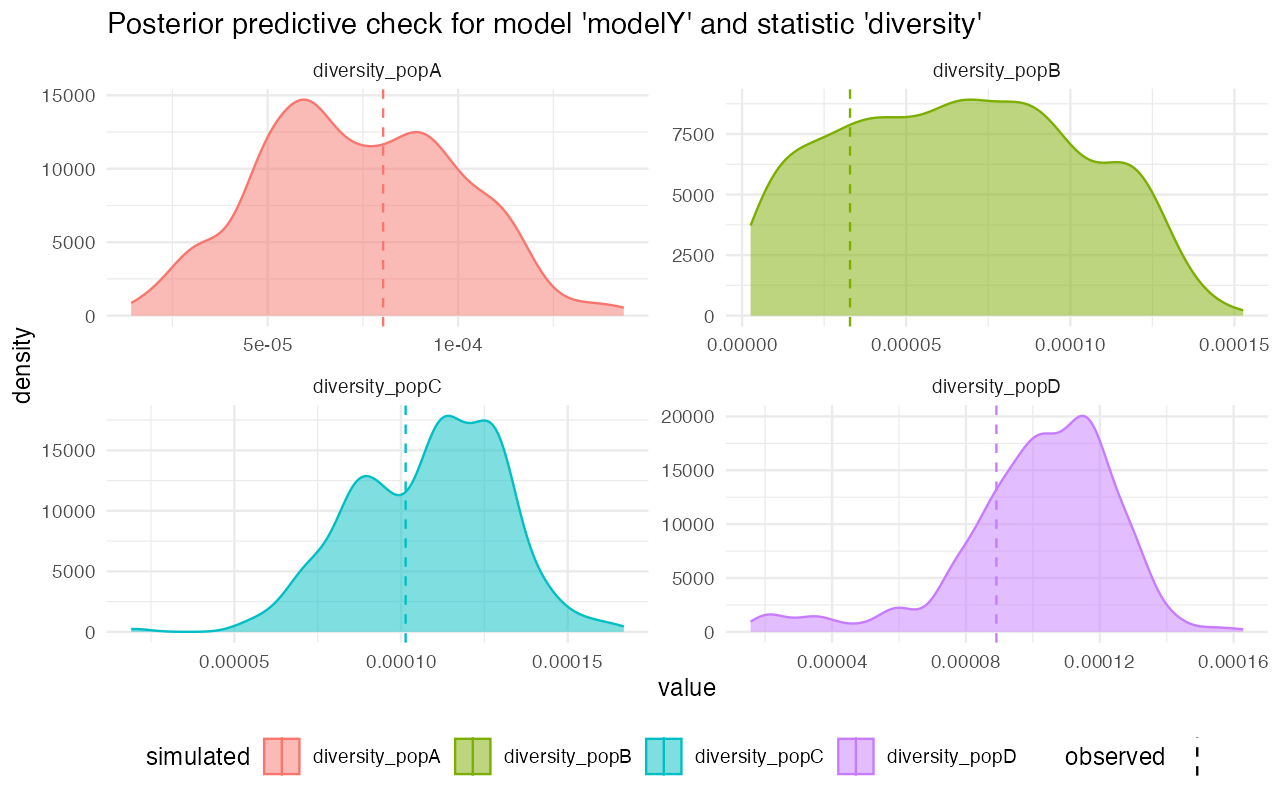

#> 
#> $divergence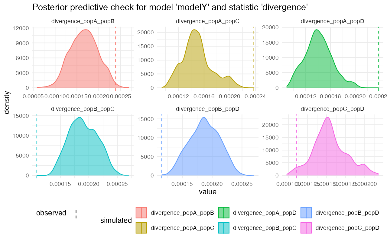

#> 
#> $f4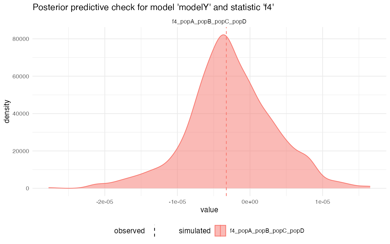

We can compare the divergences between models directly to see which model gives the most reasonable posterior predictive check results more clearly:

cowplot::plot_grid(
  plot_prediction(predX, "divergence"),
  plot_prediction(predY, "divergence"),
  plot_prediction(predZ, "divergence"),
  ncol = 1
)

We can see that posterior predictive checks for nucleotide diversity are a little less clear as there are no extremely dramatic outliers as it’s the case for divergence above:

cowplot::plot_grid(
  plot_prediction(predX, "diversity"),
  plot_prediction(predY, "diversity"),
  plot_prediction(predZ, "diversity"),
  ncol = 1
)

cowplot::plot_grid(
  plot_prediction(predX, "f4"),
  plot_prediction(predY, "f4"),
  plot_prediction(predZ, "f4"),
  ncol = 1
)

If more customization or a more detailed analyses is needed, you can also extract data from the posterior simulations themselves:

extract_prediction(predX, "diversity")

#> $diversity
#> # A tibble: 4,000 × 12
#>      rep   T_1   T_2   T_3     gf  Ne_A  Ne_B  Ne_C  Ne_D summary  stat    value
#>    <int> <dbl> <dbl> <dbl>  <dbl> <dbl> <dbl> <dbl> <dbl> <chr>    <chr>   <dbl>
#>  1     1 1218. 6392. 9831. 0.0627 1573.  987. 5493. 5879. diversi… dive… 5.89e-5
#>  2     1 1218. 6392. 9831. 0.0627 1573.  987. 5493. 5879. diversi… dive… 3.98e-5
#>  3     1 1218. 6392. 9831. 0.0627 1573.  987. 5493. 5879. diversi… dive… 9.35e-5
#>  4     1 1218. 6392. 9831. 0.0627 1573.  987. 5493. 5879. diversi… dive… 9.48e-5
#>  5     2  962. 5053. 6577. 0.0747 1105. 1215. 3420. 3951. diversi… dive… 4.94e-5
#>  6     2  962. 5053. 6577. 0.0747 1105. 1215. 3420. 3951. diversi… dive… 4.98e-5
#>  7     2  962. 5053. 6577. 0.0747 1105. 1215. 3420. 3951. diversi… dive… 9.83e-5
#>  8     2  962. 5053. 6577. 0.0747 1105. 1215. 3420. 3951. diversi… dive… 1.02e-4
#>  9     3  345. 4826. 9959. 0.294   473.  679. 7349. 6138. diversi… dive… 1.62e-5
#> 10     3  345. 4826. 9959. 0.294   473.  679. 7349. 6138. diversi… dive… 2.53e-5
#> # ℹ 3,990 more rows

However, note that extract_prediction is a convenience function which only unnests, reformats, and renames the list-columns with summary statistics stored in the predictions data frame above. You can do all the processing based on the predictions object above.

Posterior predictive checks using new statistics

In situations in which you might be interested in performing a posterior predictive check using a different set of statistics rather than the summary statistics used in the posterior inference in the first phase of your workflow (see, for instance, this discussion and associated references for more detail on why this might or might not be a valuable thing to do), you can use the optional argument functions = of the function predict(). Just like any other instances of this argument in functions such as simulate_abc(), this argument specifies a named list of summary functions. You can then compare the posterior predictions of these new summary statistics. Of course, as discussed in the link above, this might be easier said than done in practice because when we do ABC, we should be already using the best summary statistics we can, but it’s worth mentioning this possibility here for cases in which this might be relevant.

For instance, let’s say that our new summary statistics are AFS vectors in each of our four populations, which can be computed by the following tree-sequence summary statistics in R:

afs_functions <- list(
  afs_A = function(ts) { samples <- ts_names(ts, split = "pop")["A"]; ts_afs(ts, sample_sets = samples) },
  afs_B = function(ts) { samples <- ts_names(ts, split = "pop")["B"]; ts_afs(ts, sample_sets = samples) },
  afs_C = function(ts) { samples <- ts_names(ts, split = "pop")["C"]; ts_afs(ts, sample_sets = samples) },
  afs_D = function(ts) { samples <- ts_names(ts, split = "pop")["D"]; ts_afs(ts, sample_sets = samples) }
)

Again, it’s always useful to sanity check our functions definitions, which we do it by computing these statistics from a single simulated tree sequence (we make it tiny to make things faster—the point is to test whether our new summary statistics functions even run the way we want them to):

ts <- simulate_model(modelX, priors, sequence_length = 1e6, recombination_rate = 0, mutation_rate = 1e-8)

summarise_data(ts, afs_functions)

#> $afs_A
#>   [1] 2357  272   94   33   39   28   84    6   20    3   56   10    4    0    4
#>  [16]   24    4    0    3    0    0    0    0    0    3   35    0    0    0   17
#>  [31]    0    0    0    0    0    0    0    0    0    0    0    0    0    0    0
#>  [46]    0    0    0    0    0    8    0    0    0    0    0    0    0    0    0
#>  [61]    0    0    0    0    0    0    0    0    0    0    0    0    0    0    0
#>  [76]    0    0    0    0   55    0    0    0    0    0    0    0    0    0    0
#>  [91]    0    0    0    0   23    0    0    0    0    0   34
#> 
#> $afs_B
#>   [1] 2530   93   84   37    8   26    6   11   24    6   19    9    1    2    0
#>  [16]    1    0    0    0   23  117    0    0    0    0    0    0    0    0  103
#>  [31]   17    0   18    0    0    0    0    0    0    0    0    0    0    0    0
#>  [46]    0    0    0    0    0    0   47    0    0    0    0    0    0    0    0
#>  [61]    0    0    0    0    0    0    0    0    0    0    0    0    0    0    0
#>  [76]    0    0    0    0    0   25    0    0    0    0    0    0    0    0    0
#>  [91]    0    0    0    0    0    0    0    0    0    0    9
#> 
#> $afs_C
#>   [1] 2061  245  199   28   38  164   20  148   15   43    0    0    0    0    5
#>  [16]    5    0    0    0    2    0    0    2   17   10   15    0    0    0    0
#>  [31]   14   92    0    0    0    0    0    0    0    0    0    0    0    0    0
#>  [46]    0    0    0   43    0    0    0    0   16    0    0    0    0    0    0
#>  [61]    0    0   25    0    0    0    0    0    0    9    0    0    0    0    0
#>  [76]    0    0    0    0    0    0    0    0    0    0    0    0    0    0    0
#>  [91]    0    0    0    0    0    0    0    0    0    0    0
#> 
#> $afs_D
#>   [1] 2174  255  135  106   50   62   70    8   22    9    0    0   71    2    9
#>  [16]    7    0    8   10    0    6   24    0   11    0    0   60    0    0    0
#>  [31]    2    0    5    0    0    0    0    0    0    0    0    0    0    0    0
#>  [46]    0    0    0    0    0    0    0    6    0    0    0   25    0    0    0
#>  [61]    0    0    0    0    0    0    0    0    5    0    0    0    0    0   40
#>  [76]    0    0    0    0    0    0    0    0    0    0    0    0    0    0    0
#>  [91]    0    0    0    0    0    0    0    0    0    0   34

Now we can finally get the posterior predictive distributions of the new summary statistics (per-population AFS vectors), which are again stored as nested list-columns:

plan(multisession, workers = availableCores())

# we simulate only 10 samples from the posterior distribution, but this is only
# to save computational time!
pred_afs <- predict(abcX, samples = 10, posterior = "unadj", functions = afs_functions)

This means that each of those afs_... list columns contains an AFS for the corresponding population for each given replicate:

pred_afs

#> # A tibble: 10 × 13
#>      rep    T_1   T_2   T_3     gf  Ne_A  Ne_B  Ne_C  Ne_D afs_A  afs_B  afs_C 
#>    <int>  <dbl> <dbl> <dbl>  <dbl> <dbl> <dbl> <dbl> <dbl> <list> <list> <list>
#>  1     1 3050.  7577. 8936. 0.0663 2365. 1222. 3197. 2109. <dbl>  <dbl>  <dbl> 
#>  2     2   40.4 7205. 8641. 0.669  1333. 1531. 3170. 6227. <dbl>  <dbl>  <dbl> 
#>  3     3 1538.  4675. 9914. 0.642  1456.  664. 5659. 4147. <dbl>  <dbl>  <dbl> 
#>  4     4 2373.  6711. 9685. 0.688  2019. 1263. 9451. 4505. <dbl>  <dbl>  <dbl> 
#>  5     5  967.  8902. 9671. 0.886  1851. 2284. 3933.  589. <dbl>  <dbl>  <dbl> 
#>  6     6 1217.  5746. 5894. 0.240  1456.  294. 6053. 4875. <dbl>  <dbl>  <dbl> 
#>  7     7 2758.  8007. 9034. 0.524  2810. 1341. 5109. 8394. <dbl>  <dbl>  <dbl> 
#>  8     8 3094.  7611. 7852. 0.0949 1701. 1381. 7170. 7504. <dbl>  <dbl>  <dbl> 
#>  9     9 2167.  7024. 9708. 0.261  1497. 1886. 3156. 4523. <dbl>  <dbl>  <dbl> 
#> 10    10 1644.  5518. 9061. 0.0186 2032.  864. 4695. 1399. <dbl>  <dbl>  <dbl> 
#> # ℹ 1 more variable: afs_D <list>

Here’s one of them for the population “A” and the first simulated posterior sample:

pred_afs[1, ]$afs_A

#> [[1]]
#>   [1] 10165  1073   465   309   232   199   191   153   124   126   102   110
#>  [13]   108   110    79    90    60    62    59    57    62    56    38    47
#>  [25]    43    36    41    40    28    26    25    33    34    40    30    28
#>  [37]    24    19    19    33    33    23    18    27    13    20    19    15
#>  [49]    29    19    14    15    20    13    20    15    11    19    19    28
#>  [61]    21    12     8     9    13    23     8    16     8    23    11    25
#>  [73]    13     6    15    17     6    16    18    10    14    17    11     9
#>  [85]    11    22    11    20    16    15    11    11     7    13    14     3
#>  [97]     4     2    12    11   320

Additional diagnostics and backwards compatibility with the abc package

As mentioned above, the functionality behind cross_validate() is implemented by reformatting the results of demografr simulation and inference functionality in a form necessary to run the functions of the abc package cv4abc() and cv4postpr() behind the scenes – a task that normally requires a significant amount of potentially error-prone bookkeeping on part of the user.

In addition to demografr’s own function predict() which implements posterior predictive checks, the abc package provides additional functionality for evaluating the quality of the fit of an ABC model to the data, namely gfit() and gfitpca(). In this section we demonstrate how this functionality (and potentially other future abc functions) can be applied on demografr data with very little additional work.

First, demografr provides a function unpack() which – when applied on an object generated either by simulate_abc() or run_abc() – unpacks the object encapsulating all information describing the simulation and inference which produced it, into individual components with names matching the “low-level” function arguments of all relevant functions of the anc package. This includes gfit() and gfitpca() mentioned above, but also functions cv4abc() and cv4postpr(). Here is how unpack() works.

“Unpacking” a demografr object to low-level components used by the abc package

partsX <- unpack(abcX)

class(partsX)

#> [1] "list"

names(partsX)

#> [1] "sumstat" "index"   "param"   "target"

As we can see, the unpack() function produced a list object with several elements. It’s not a coincidence that the names of these list elements correspond to function arguments of various diagnostic functions of the abc package. In this way, demografr pre-generates the information required by those functions (which normally need to be prepared manually), which can then be run without any additional work whatsoever. For instance, we could perform the cross-validation of the model selection using abc’s own functionality like this.

First, because model-selection requires, well, multiple models to select from, we will unpack information from all the three models:

parts <- unpack(list(abcX, abcY, abcZ))

class(parts)

#> [1] "list"

names(parts)

#> [1] "sumstat" "index"   "param"   "target"

Then, we simply run cv4postpr() as we normally would, using the information pre-generated by unpack():

library(abc) # cv4postpr() is a function from the abc R package, not demografr!

cv4postpr_res <- cv4postpr(index = parts$index, sumstat = parts$sumstat, nval = 10, tols = 0.01, method = "neuralnet")

Unlike the result of cross_validate() above, typing out the object cv4postpr_res will not help us, but we can get the overview of the results by applying the function summary():

summary(cv4postpr_res)

#> Confusion matrix based on 10 samples for each model.
#> 
#> $tol0.01
#>        modelX modelY modelZ
#> modelX     10      0      0
#> modelY      0     10      0
#> modelZ      0      0     10
#> 
#> 
#> Mean model posterior probabilities (neuralnet)
#> 
#> $tol0.01
#>        modelX modelY modelZ
#> modelX 0.9193 0.0640 0.0167
#> modelY 0.0294 0.9635 0.0071
#> modelZ 0.0003 0.0199 0.9799

As you can see, we can replicate the result of cross_validate() for model selection by combining the functions unpack(), cv4postpr() and summary(). Of course, using cross_validate() allows us to do this all in one go in a straightforward way, but the above hopefully demonstrates that there’s no magic behind demografr’s convenient functionality. It just streamlines the process of ABC diagnostics and avoids unnecessary (and potentially error-prone) data processing.

On a similar note, we can also run abc functions gfit() and gfitpca() (as described in this vignette) in exactly the same way. We will focus just on the code, and leave the interpretation to the discussion in the vignette:

First, we will unpack the results of the selected best-fitting model from the appropriate abc object obtained by the demografr function run_abc() above:

partsX <- unpack(abcX)

class(partsX)

#> [1] "list"

names(partsX)

#> [1] "sumstat" "index"   "param"   "target"

Then we use the elements of the parts list that we just created as inputs for gfit():

library(abc) # gfit() is a function from the abc R package, not demografr!

gfitX <- gfit(target = partsX$target, sumstat = partsX$sumstat, statistic = mean, nb.replicate = 100)

plot(gfitX, main="Histogram under H0 (model X)")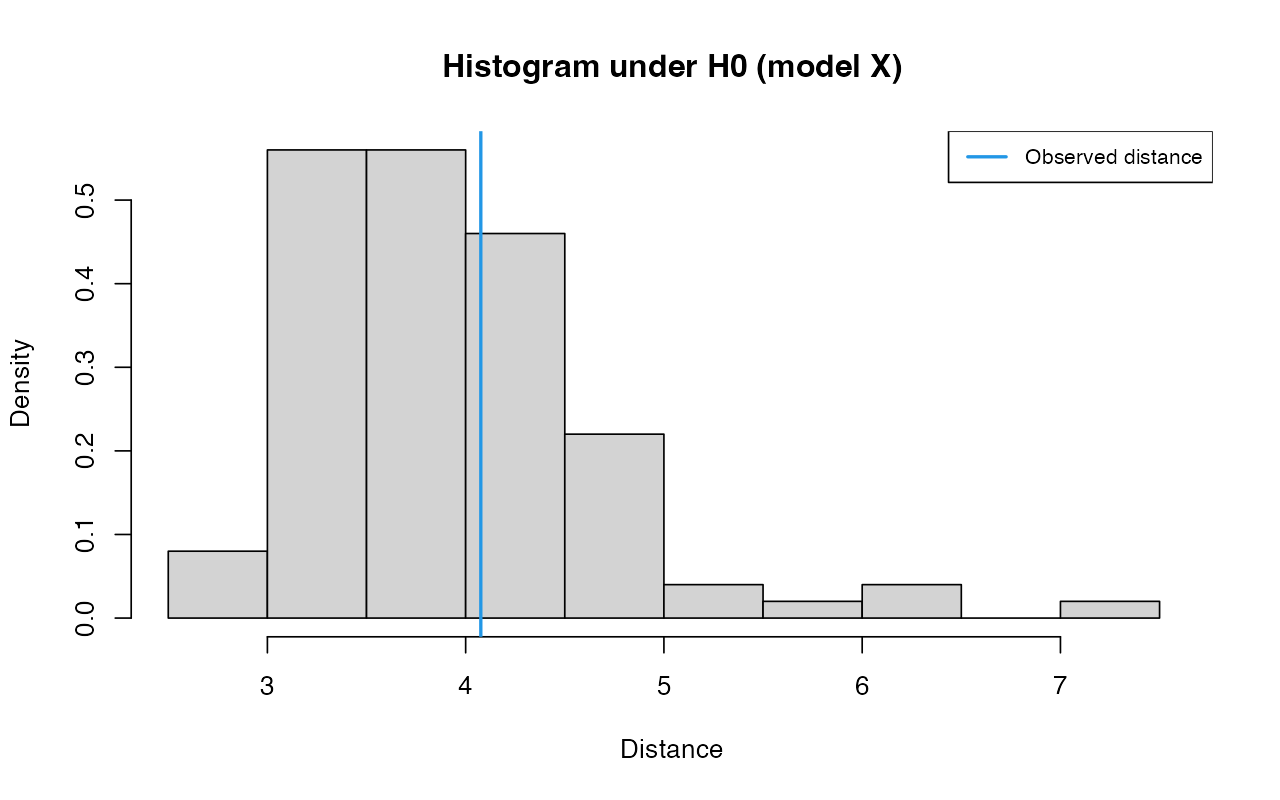

summary(gfitX)

#> $pvalue
#> [1] 0.35
#> 
#> $s.dist.sim
#>    Min. 1st Qu.  Median    Mean 3rd Qu.    Max. 
#>   2.958   3.462   3.822   3.959   4.384   5.866 
#> 
#> $dist.obs
#> [1] 4.076438

partsY <- unpack(abcY)

gfitY <- gfit(target = partsY$target, sumstat = partsY$sumstat, statistic = mean, nb.replicate = 100)

plot(gfitY, main="Histogram under H0 (model Y)")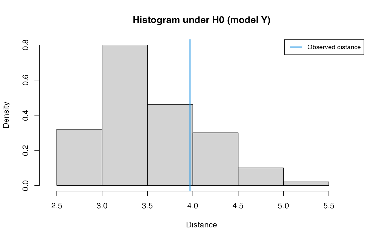

summary(gfitY)

#> $pvalue
#> [1] 0.22
#> 
#> $s.dist.sim
#>    Min. 1st Qu.  Median    Mean 3rd Qu.    Max. 
#>   2.703   3.086   3.423   3.532   3.904   4.941 
#> 
#> $dist.obs
#> [1] 3.968966

partsZ <- unpack(abcZ)

gfitZ <- gfit(target = partsZ$target, sumstat = partsZ$sumstat, statistic = mean, nb.replicate = 100)

plot(gfitZ, main="Histogram under H0 (model Z)")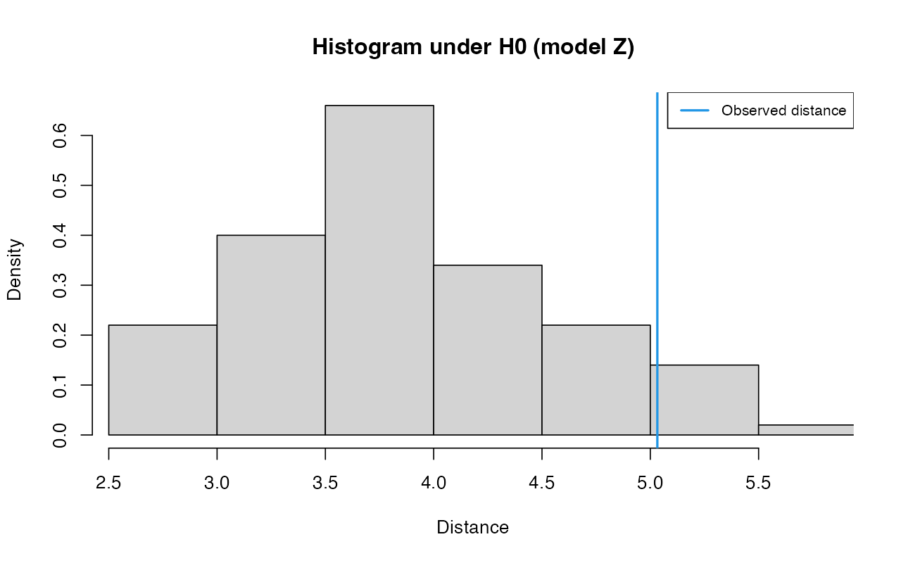

summary(gfitZ)

#> $pvalue
#> [1] 0.07
#> 
#> $s.dist.sim
#>    Min. 1st Qu.  Median    Mean 3rd Qu.    Max. 
#>   2.942   3.268   3.733   3.853   4.384   5.915 
#> 
#> $dist.obs
#> [1] 5.032494

For completeness, here is how we can run gfitpca() on demografr results:

library(abc) # gfitpca() is a function from the abc R package, not demografr!

parts <- unpack(list(abcX, abcY, abcZ))

# this needs to be loaded because of a bug in abc dependency handling
library(locfit)
gfitpca(target = parts$target, sumstat = parts$sumstat, index = parts$index, cprob = 0.01,
        xlim = c(-7, 7), ylim = c(-6, 3))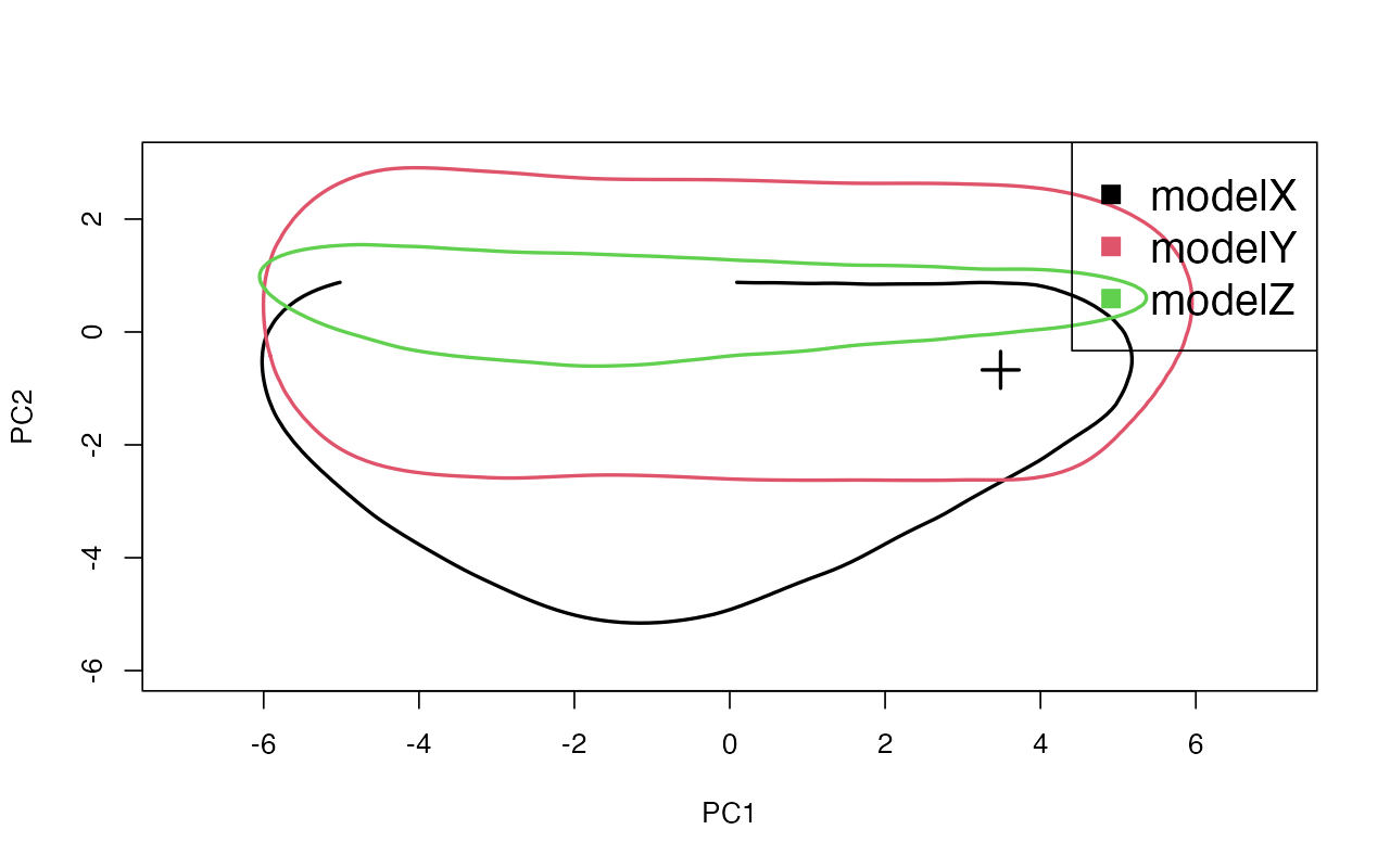

Based on the PCA, it appears that although model X and model Y are able to generate summary statistics (the areas captured by the colored “envelopes” in 2D space) compatible with the observed values (the cross), modelZ clearly cannot.

ABC cross-validation

Now we are finally at a point at which we can infer the parameters of our model against the data. However, before we do so, we should first check if our ABC setup can even estimate the model parameters at all. As we have seen just above, the abc package provides a ABC cross-validation function cv4abc() for which demografr implements a convenient interface in the form of the method cross_validate(). Above we have seen how to use this method to perform model selection, if given a list of multiple ABC objects as input. Instead, if given a single demografr ABC object (generated by the function run_abc()), it performs ABC cross-validation which we can use to gauge the accuracy of ABC and the sensitivity of the parameter estimates to the tolerance rate.

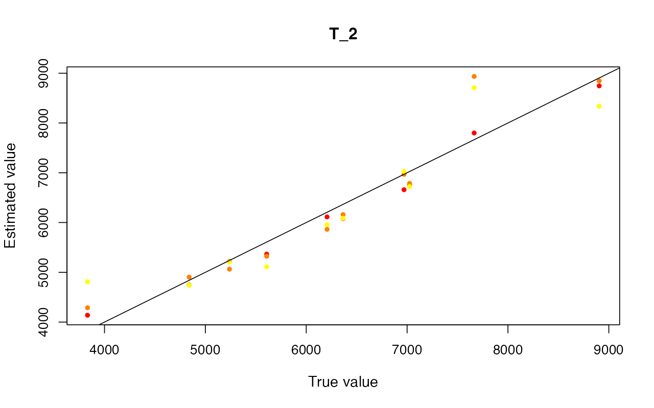
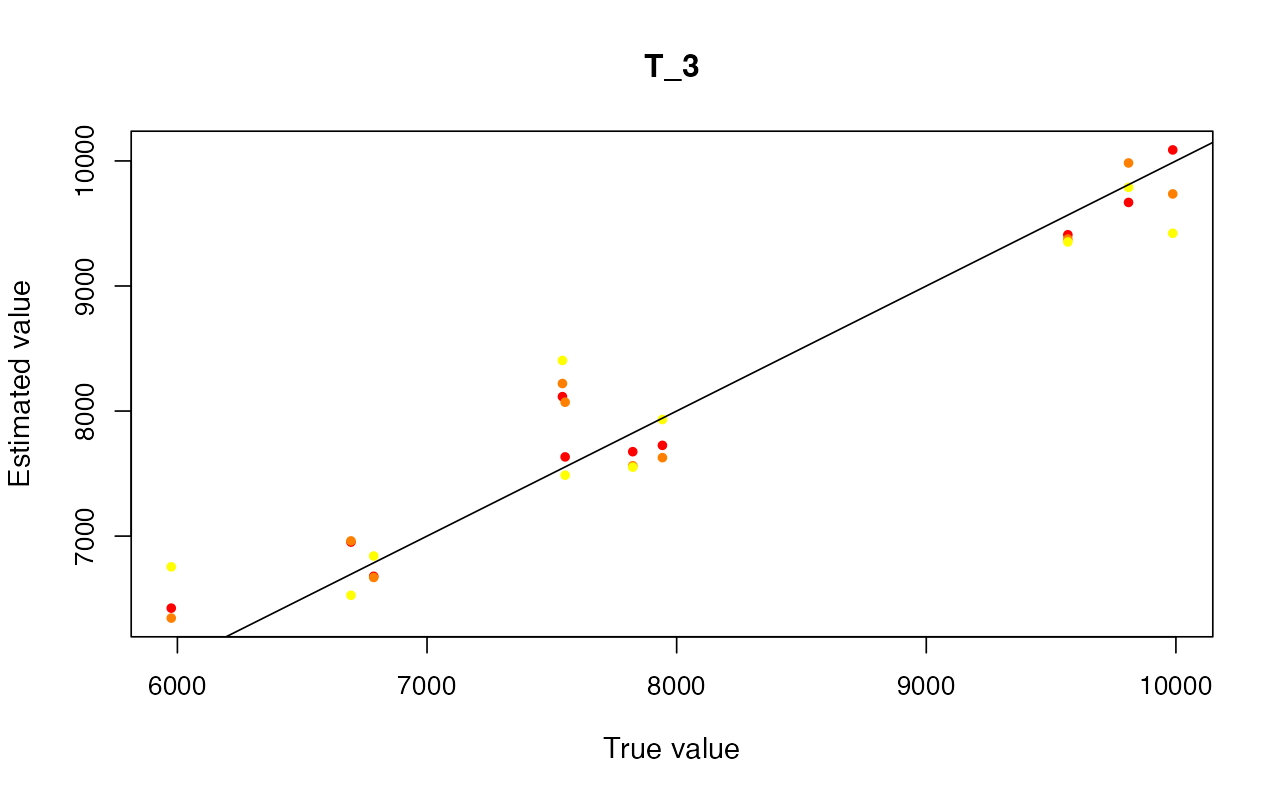
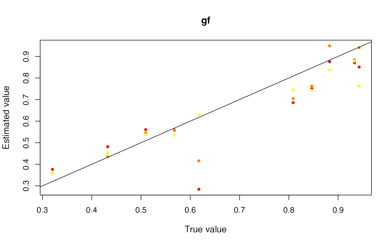
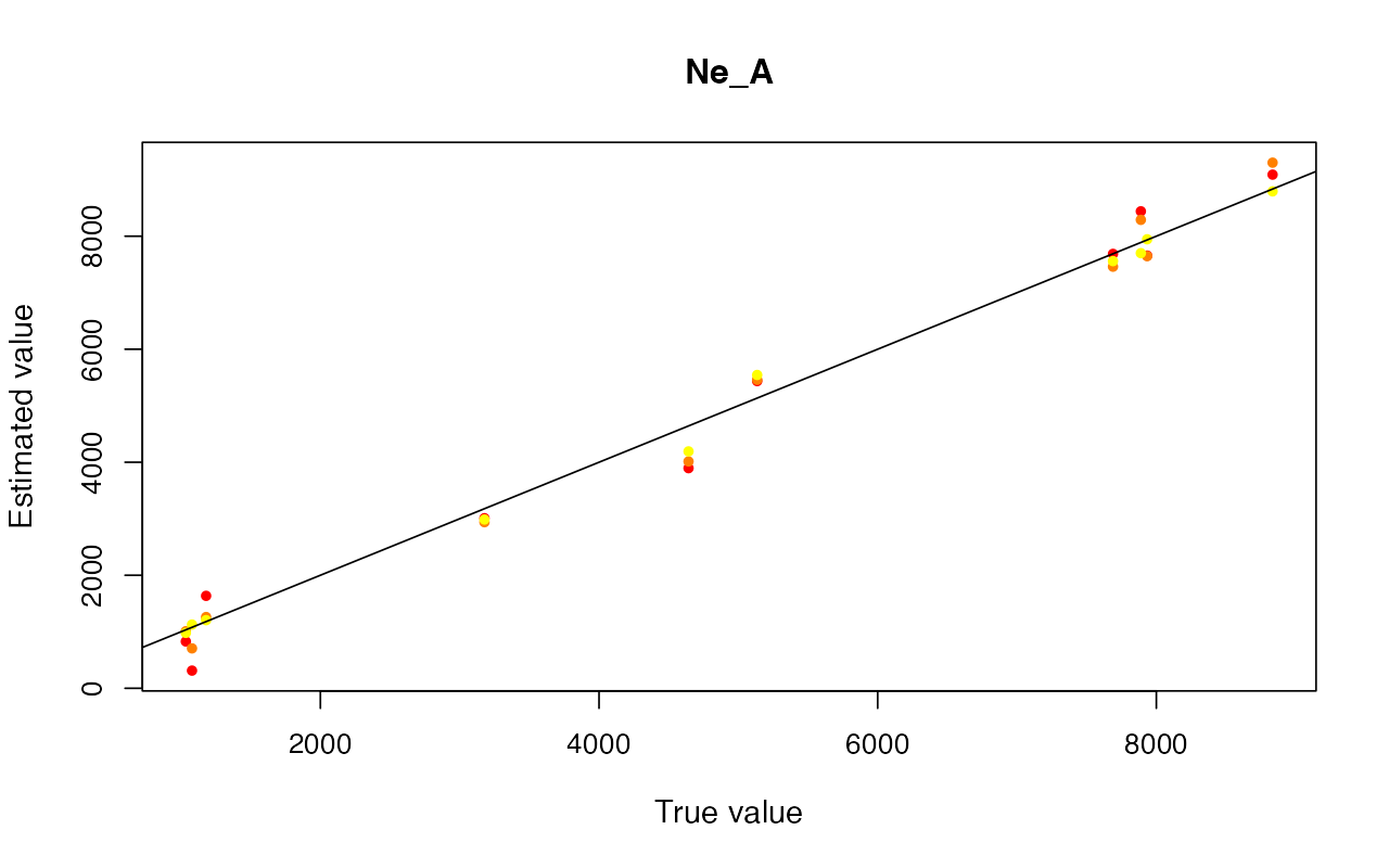
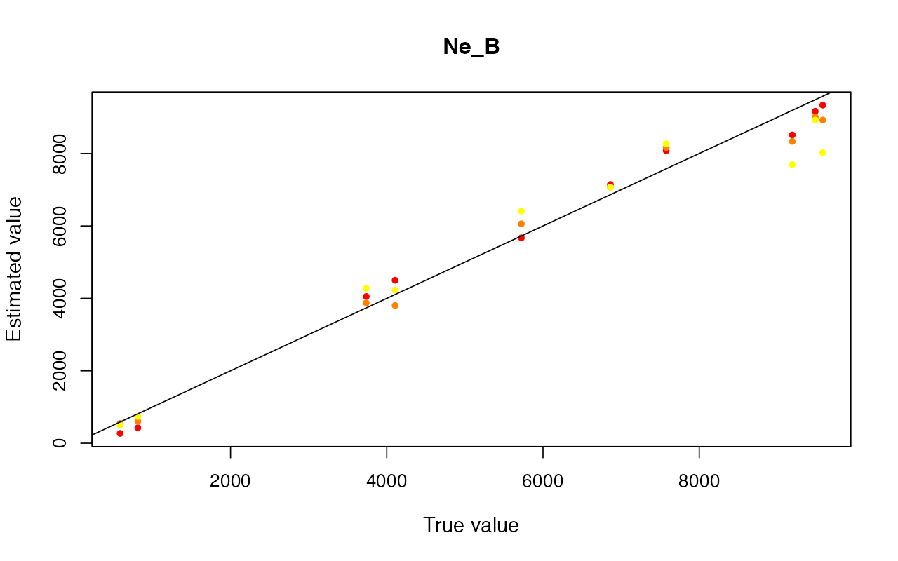
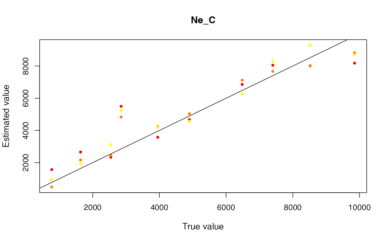
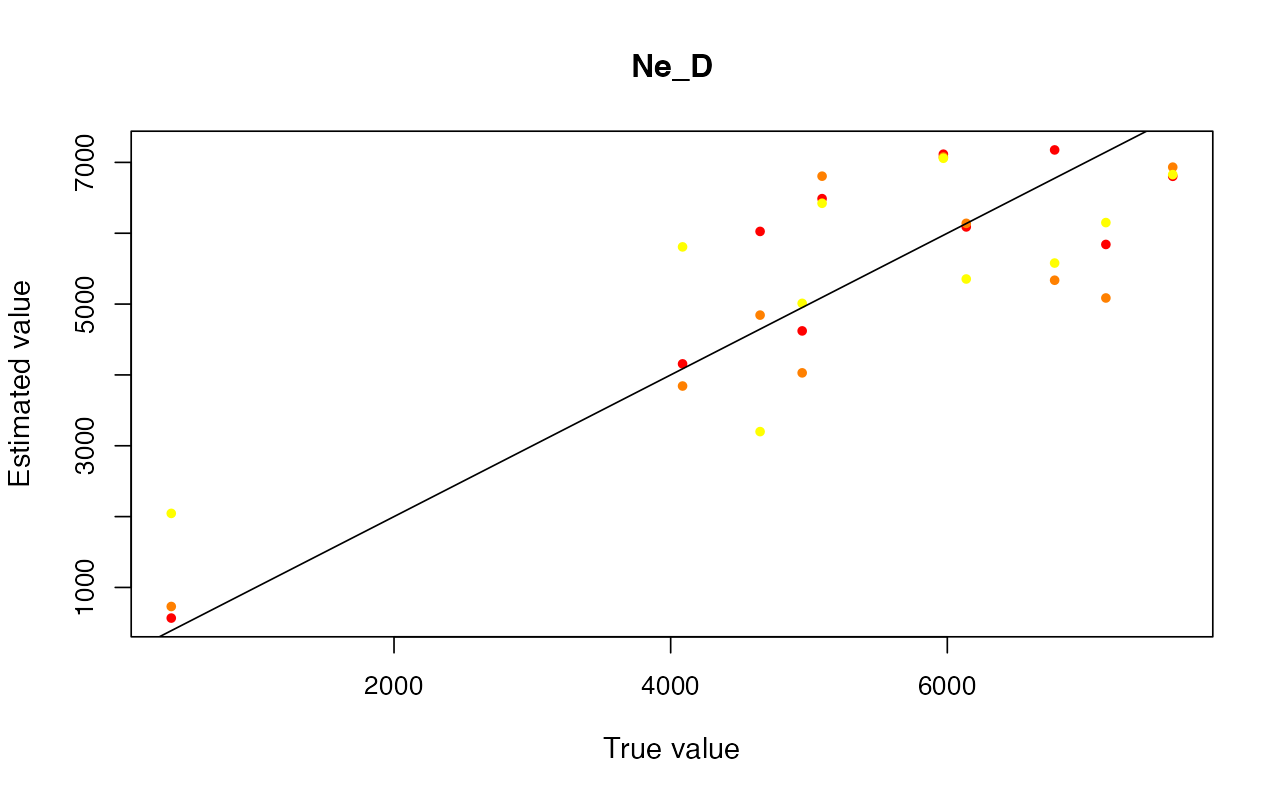
cv_abc <- cross_validate(abcX, nval = 10, tols = c(0.005, 0.01, 0.05), method = "neuralnet")
cv_abc_loclinear <- cross_validate(abcX, nval = 10, tols = c(0.005, 0.01, 0.05), method = "loclinear")
cv_abc_rejection <- cross_validate(abcX, nval = 10, tols = c(0.005, 0.01, 0.05), method = "rejection")

cv_abc

#> Prediction error based on a cross-validation sample of 10
#> 
#>               T_1         T_2         T_3          gf        Ne_A        Ne_B
#> 0.005 0.066127677 0.059804264 0.127565665 0.176387818 0.016653242 0.033635941
#> 0.01  0.076075754 0.028500770 0.055767416 0.238912106 0.009378181 0.021096094
#> 0.05  0.054353933 0.062892707 0.113332733 0.330300985 0.026141790 0.087732732
#>              Ne_C        Ne_D
#> 0.005 0.425600692 0.268586461
#> 0.01  0.330747722 0.210105302
#> 0.05  0.296105927 0.171603983

plot(cv_abc)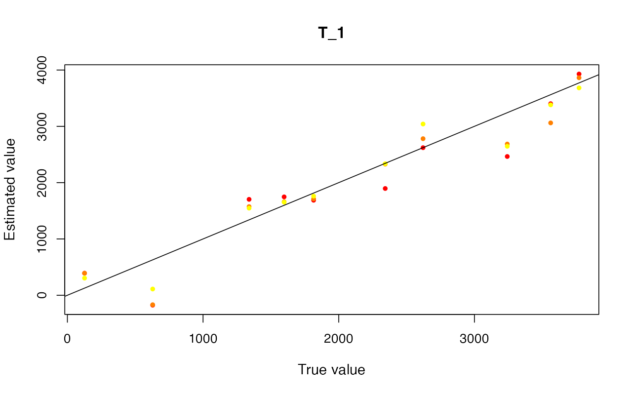

Parameter inference

Now we can finally estimate the model parameters from the model which seems to explain data the best – modelX. Because we simulated the data from a (hidden) true, known model, we will also visualize the true parameter values as vertical dashed lines to compare their values against the posterior distributions of all parameters.

abcX

#> Call:
#> abc::abc(target = observed, param = data$parameters, sumstat = simulated, 
#>     tol = 0.01, method = "neuralnet")
#> Method:
#> Non-linear regression via neural networks
#> with correction for heteroscedasticity
#> 
#> Parameters:
#> T_1, T_2, T_3, gf, Ne_A, Ne_B, Ne_C, Ne_D
#> 
#> Statistics:
#> diversity_A, diversity_B, diversity_C, diversity_D, divergence_A_B, divergence_A_C, divergence_A_D, divergence_B_C, divergence_B_D, divergence_C_D, f4_A_B_C_D
#> 
#> Total number of simulations 10000 
#> 
#> Number of accepted simulations:  100

extract_summary(abcX)

#> Warning in density.default(x, weights = weights): Selecting bandwidth *not*
#> using 'weights'
#> Warning in density.default(x, weights = weights): Selecting bandwidth *not*
#> using 'weights'
#> Warning in density.default(x, weights = weights): Selecting bandwidth *not*
#> using 'weights'
#> Warning in density.default(x, weights = weights): Selecting bandwidth *not*
#> using 'weights'
#> Warning in density.default(x, weights = weights): Selecting bandwidth *not*
#> using 'weights'
#> Warning in density.default(x, weights = weights): Selecting bandwidth *not*
#> using 'weights'
#> Warning in density.default(x, weights = weights): Selecting bandwidth *not*
#> using 'weights'
#> Warning in density.default(x, weights = weights): Selecting bandwidth *not*
#> using 'weights'

#>                             T_1      T_2      T_3          gf      Ne_A
#> Min.:                  1462.618 3030.968 6617.586 -0.10991103  679.2167
#> Weighted 2.5 % Perc.:  1517.251 4319.252 7180.513 -0.07031312  890.9708
#> Weighted Median:       2148.144 5806.244 8460.379  0.12172614 2083.5104
#> Weighted Mean:         2128.986 5730.303 8432.278  0.14010521 2093.5091
#> Weighted Mode:         2217.808 5909.163 8424.770  0.10064241 1955.3505
#> Weighted 97.5 % Perc.: 2718.882 6404.353 9286.605  0.41296552 3102.2050
#> Max.:                  3030.757 6599.029 9532.209  0.64394792 4300.4994
#>                             Ne_B      Ne_C      Ne_D
#> Min.:                   274.4861  1251.380 -2265.807
#> Weighted 2.5 % Perc.:   338.0007  3580.354 -1039.344
#> Weighted Median:        856.8090  6934.996  2494.683
#> Weighted Mean:          881.8393  6803.139  2724.711
#> Weighted Mode:          857.0188  7408.730  2077.874
#> Weighted 97.5 % Perc.: 1482.2222 11379.856  6714.054
#> Max.:                  1578.6224 12019.281  7547.764

library(ggplot2)

plot_posterior(abcX, param = "T") +
  geom_vline(xintercept = c(2000, 6000, 8000), linetype = "dashed")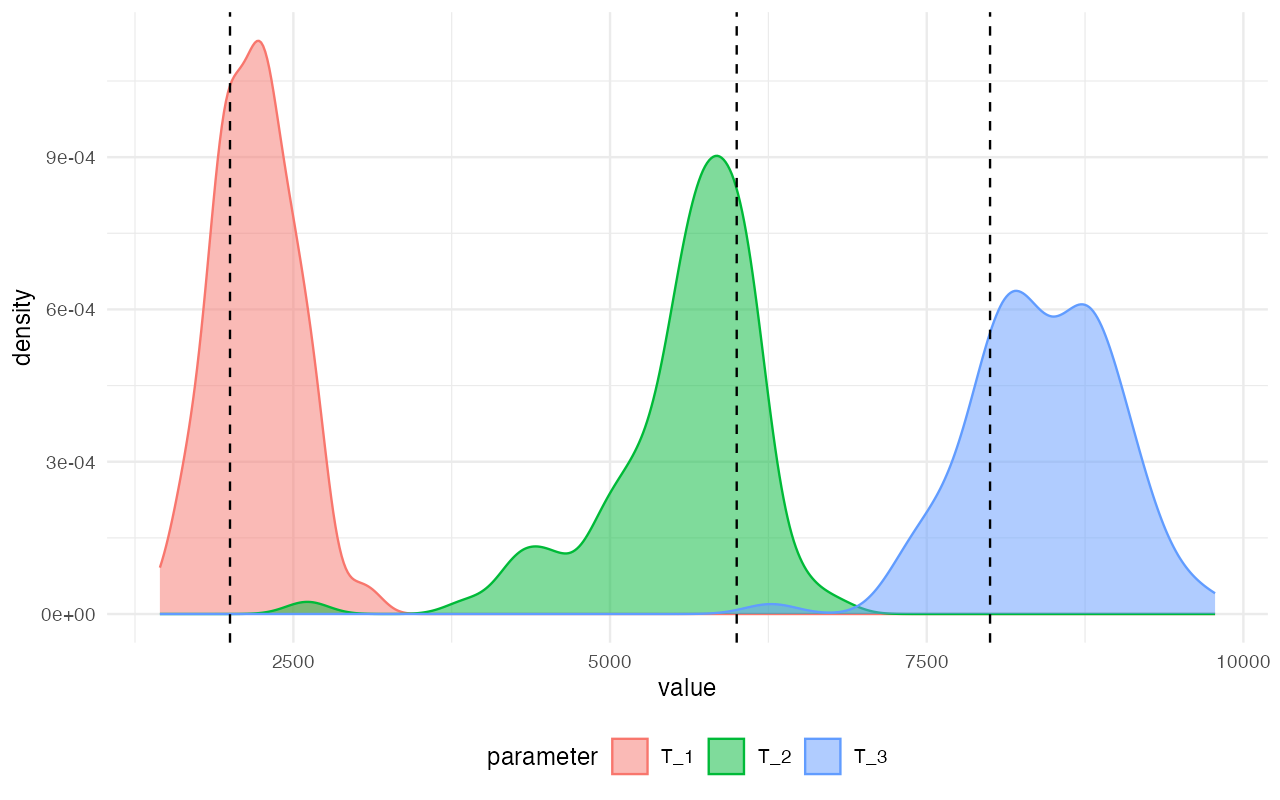

plot_posterior(abcX, param = "Ne") +
    geom_vline(xintercept = c(2000, 800, 9000, 4000), linetype = "dashed")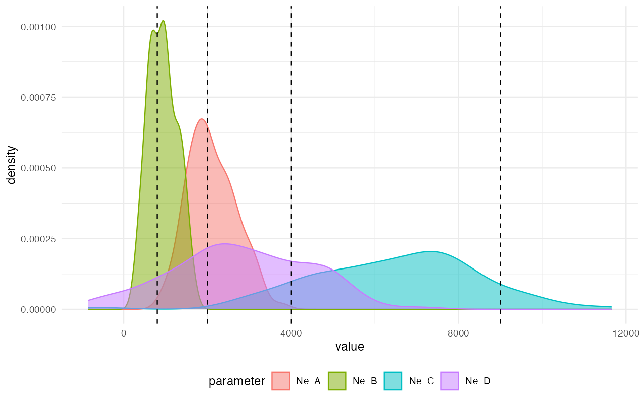

plot_posterior(abcX, param = "gf") +
  geom_vline(xintercept = 0.1, linetype = "dashed") +
  coord_cartesian(xlim = c(0, 1))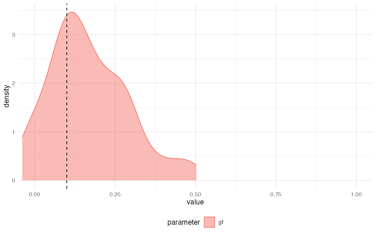

Not bad, considering how few simulations we’ve thrown at the inference in order to save computational resources in this small vignette! We can see that the modes of the inferred posterior distributions of the model parameters (the colorful densities plotted above) line up pretty much perfectly with the true values (dashed vertical lines).

To make this concluding point even clearer (and also to demonstrate the importance of the various validation procedures described above, such as the posterior predictive checks!) let’s say that we weren’t careful enough with model selection and simply assumed that the structure of modelZ is the most appropriate model for our data and used it for inference of the split time parameters instead. This is complete non-sense and we show this purely for demonstration purposes!

plot_posterior(abcZ, param = "T") +
  geom_vline(xintercept = c(2000, 6000, 8000), linetype = "dashed")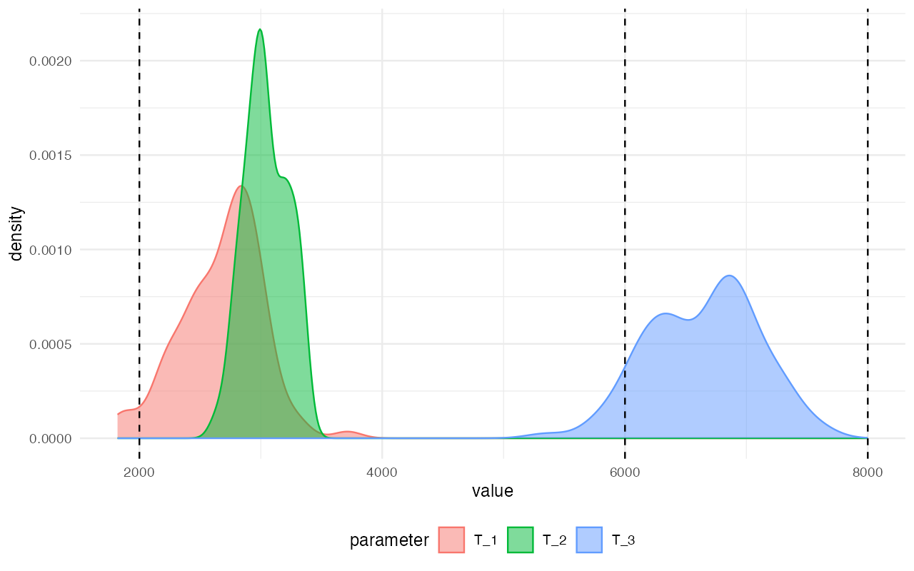

We can clearly see that posterior distributions inferred by ABC for this particular model completely failed to capture the true values.