Custom inference using SLiM or Python
Source:vignettes/vignette-05-custom.Rmd
vignette-05-custom.Rmd⚠️⚠️⚠️
Please note that until a peer reviewed publication describing the demografr package is published, the software should be regarded as experimental and potentially unstable.
⚠️️⚠️⚠️
By default, demografr uses the slendr package for defining models and simulating data from them. But what if you need to do inference using your own scripts? Perhaps slendr’s opinionated interface doesn’t allow you to do all that you need to do, such as using some of the powerful simulation features and options of “raw” SLiM or msprime? Alternatively, perhaps you don’t want to compute summary statistics (just) with slendr’s tree-sequence interface to tskit (you might want to compute statistics using other software), or you want to compute statistics with fully customized Python functions. This vignette explains how you can use any standard SLiM or msprime script as a simulation engine in a standard demografr pipeline without slendr, as well as how to utilize customized, non-slendr summary statistic functions.
First, let’s load demografr itself and also slendr (which, in this vignette, will serve only for working with simulated tree sequences, but not simulations themselves).
Toy inference problem
Suppose that we intent to use ABC to infer the of a constant-sized population given that we observed the following value of nucleotide diversity:
observed_diversity#> # A tibble: 1 × 2
#> set diversity
#> <chr> <dbl>
#> 1 pop 0.0000394We want to infer the posterior distribution of . In this vignette, we’re going to show how to accomplish first not via the normal slendr interface (as shown here) but using a simple SLiM or Python script. In a later section, we’re also going to use this example to demonstrate how to compute population genetic summary statistic (like nucleotide diversity) using external software.
We acknowledge that this is a completely trivial example, not really worth spending so much effort on doing an ABC for. The example was chosen because it runs fast and demonstrates all the features of demografr that you would use regardless of the complexity of your model.
Using custom scripts as simulation engines
In order to be able to use a custom SLiM or msprime script with demografr, the script must conform to a couple of rules:
1. It must be runnable on the command-line as any other command-line script
For an msprime script, this means something like
python <your script>.py <command-line arguments>.For a SLiM script, this means something like
slim <command-line arguments> <your script>.slim.
2. It must accept --path argument pointing to a
directory where it will save output files
This is analogous to the path = argument of
slendr functions slim() and
msprime().
For an msprime script, this parameter can
be specified via the Python built-in module argparse, and
provided on the command-line as
--path <path to directory>. In the script itself, if
you use the argparse module and have thus the values of
provided arguments (for instance) in an args object, you
can then refer to these arguments as args.path, etc. Given
that you’re reading this, I assume you know what the above information
means, but here’s a link to the
relevant section of the Python documentation for completeness.
For a SLiM script, this parameter can be specified
via SLiM’s standard way of supplying command-line arguments as
-d "path='<path to a directory>'". Importantly, note
SLiM’s format of specifying string arguments for the path
argument. If you need further detail, see Section 20.2 of the SLiM
manual. In the script itself, you can then refer to this argument via
the constant path.
3. All model parameters must be provided as additional command-line arguments
You can refer to them in your script as you would to the mandatory arguments as described in the previous section.
A useful check to see whether you script would make a valid engine for a demografr inference pipeline is to run it manually on the command line like this:
python \
  <path to your Python script>                   \
  --path <path to a directory> \
  <... your model parameters ...>
Or, if you want to run a SLiM-powered ABC, like this:
slim \
  -d "path='<path to a directory>'" \
  <... your model parameters ...>
Then, if you look into the directory and see the desired files produced by your simulation script, you’re good to go!
Below you are going to see how to actually read back
simulation results from disk and use them for computing summary
statistics. For now, just note that you can name the files produced by
your simulation script however you’d like and can have as many as you’d
like, as long as they are all in that one directory given by
path.
Example pure SLiM and msprime script
To demonstrate the requirements 1-3 above in practice, let’s run an ABC inference using an example msprime script and a SLiM script as simulation engines.
Imagine we have the following two scripts which we want to use as
simulation engines instead of slendr’s own functions
slim() and msprime(). The scripts have only
one model parameter,
of the single modeled population. The other parameters
are mandatory, just discussed in the previous section.
SLiM script
slim_script <- system.file("examples/custom.slim", package = "demografr")initialize() {
initializeTreeSeq();
initializeMutationRate(1e-8);
initializeMutationType("m1", 0.5, "f", 0.0);
initializeGenomicElementType("g1", m1, 1.0);
initializeGenomicElement(g1, 0, 1e6 - 1);
initializeRecombinationRate(1e-8);
}
1 early() {
sim.addSubpop("p0", asInteger(Ne));
}
10000 late() {
ts_path = path + "/" + "result.trees";
sim.treeSeqOutput(ts_path);
}Python script
python_script <- system.file("examples/custom.py", package = "demografr")import argparse
import msprime
parser = argparse.ArgumentParser()
# mandatory command-line argument
parser.add_argument("--path", type=str, required=True)
# model parameters
parser.add_argument("--Ne", type=float, required=True)
args = parser.parse_args()
ts = msprime.sim_ancestry(
samples=round(args.Ne),
population_size=args.Ne,
sequence_length=1e6,
recombination_rate=1e-8,
)
ts = msprime.sim_mutations(ts, 1e-8)
ts.dump(args.path + "/" + "result.trees")Note that the Python script specifies all model parameters
(here just
)
and mandatory arguments via a command-line interface provided by the
Python module argparse.
The SLiM script, on the other hand, uses SLiM’s features for command-line specification of parameters and simply refers to each parameter by its symbolic name. No other setup is necessary.
Please also note that given that there are can be discrepancies
between values of arguments of some SLiM or Python methods (such as
addSubPop of SLiM which expects an integer value for a
population size, or the samples argument of
msprime.sim_ancestry), and values of parameters sampled
from priors by demografr (i.e.,
often being a floating-point value after sampling from a continuous
prior), you might have to perform explicit type conversion in your
custom scripts (such as sim.addSubPop("p0", asInteger(Ne)
as above).
ABC inference using custom msprime script
Apart from the user-defined simulation SLiM and msprime scripts, the components of our toy inference remains the same—we need to define the observed statistics, tree-sequence summary functions, and priors. We don’t need a model function—that will be served by our custom script.
Here are the demografr pipeline components (we won’t be discussing them here because that’s extensively taken care of elsewhere in demografr’s documentation vignettes):
# a single prior parameter
priors <- list(Ne ~ runif(100, 5000))

# a single observed statistic
observed <- list(diversity = observed_diversity)

# compute diversity using 100 chromosomes
compute_diversity_ts <- function(ts) {
  samples <- ts$samples()
  ts_diversity(ts, list(pop = sample(samples, 100)))
}
functions <- list(diversity = compute_diversity_ts)

# data-generating functions for computing summary statistics
gens <- list(
  ts = function(path) ts_read(file.path(path, "result.trees"))
)
(Note that because our simulated tree sequences won’t be coming with slendr metadata, we have to refer to individuals’ chromosomes using numerical indices rather than slendr symbolic names like we do in all of our other vignettes.)
Simulating a testing tree sequence
As we explained elsewhere, a useful function for developing inference
pipelines using demografr is a function
simulate_model(), which normally accepts a slendr
model generating function and the model parameters (either given as
priors or as a list of named values), and simulates a tree-sequence
object. This function (as any other demografr function
operating with models) accepts our custom-defined simulation scripts in
place of standard slendr models.
For instance, we can simulate a couple of Mb of testing sequence from our msprime script like this:
model_run <- simulate_model(python_script, parameters = list(Ne = 123), format = "files", data = gens)Now we can finally test our toy tree-sequence summary function, verifying that we can indeed compute the summary statistic we want to:
functions$diversity(model_run$ts)#> # A tibble: 1 × 2
#> set diversity
#> <chr> <dbl>
#> 1 pop 0.00000380The function works as expected—we have a single population and want to compute nucleotide diversity in the whole population, and this is exactly what we get.
#> # A tibble: 1 × 2
#>   set    diversity
#>   <chr>      <dbl>
#> 1 pop   0.00000419
#> $diversity
#> # A tibble: 1 × 2
#> set diversity
#> <chr> <dbl>
#> 1 pop 0.00000389Note that we are also able to use a dedicated function for this,
called summarise_data(), which takes in a product of a
simulation (tree sequence and/or a path to a directory with simulation
results), and apply all summary functions to this data:
summarise_data(model_run, functions)#> $diversity
#> # A tibble: 1 × 2
#> set diversity
#> <chr> <dbl>
#> 1 pop 0.00000375ABC inference
Having all components of our pipeline set up we should, again, validate everything before we proceed to (potentially very costly) simulations. In the remainder of this vignette we’ll only continue with the Python msprime custom script in order to save some computational time. That said, it’s important to realize that you could use this sort of workflow for any kind of SLiM script, including very elaborate spatial simulations, non-WF models, and all kinds of phenotypic simulations too! Although primarily designed to work with slendr, the demografr package intends to fully support any kind of SLiM or msprime simulation. If something doesn’t work, consider it a demografr bug!
Let’s first validate all components of our pipeline:
validate_abc(python_script, priors, functions, observed, data = gens, format = "files")#> ======================================================================
#> Testing sampling of each prior parameter:
#> - Ne ✅
#> ---------------------------------------------------------------------
#> The model is a custom user-defined msprime script
#> ---------------------------------------------------------------------
#> Simulating tree sequence from the given model... ✅
#> ---------------------------------------------------------------------
#> Validating custom data-generating functions... ✅
#> ---------------------------------------------------------------------
#> Generating data from simulation results:
#> - ts (type slendr_ts) ✅
#> ---------------------------------------------------------------------
#> Computing user-defined summary functions:
#> - diversity ✅
#> ---------------------------------------------------------------------
#> Checking the format of simulated summary statistics:
#> - diversity [data frame] ✅
#> ======================================================================
#> No issues have been found in the ABC setup!Looking good! Now let’s first run ABC simulations. Again, note the
use of the Python script where we would normally provide a
slendr model function in place of the model
argument:
library(future)
plan(multisession, workers = availableCores()) # parallelize across all CPUs

data <- simulate_abc(
  model = python_script, priors, functions, observed, iterations = 10000,
  data = gens, format = "files"
)
The total runtime for the ABC simulations was 0 hours 47 minutes 44 seconds parallelized across 96 CPUs.
Once the simulations are finished, we can perform inference of the posterior distribution of the single parameter of our model, :
abc <- run_abc(data, tol = 0.01, method = "neuralnet")Having done so, we can again look at the summary statistics of the
posterior distribution and also plot the results (we’re skipping
diagnostics such as posterior predictive checks but you can read more
about those here
and here).
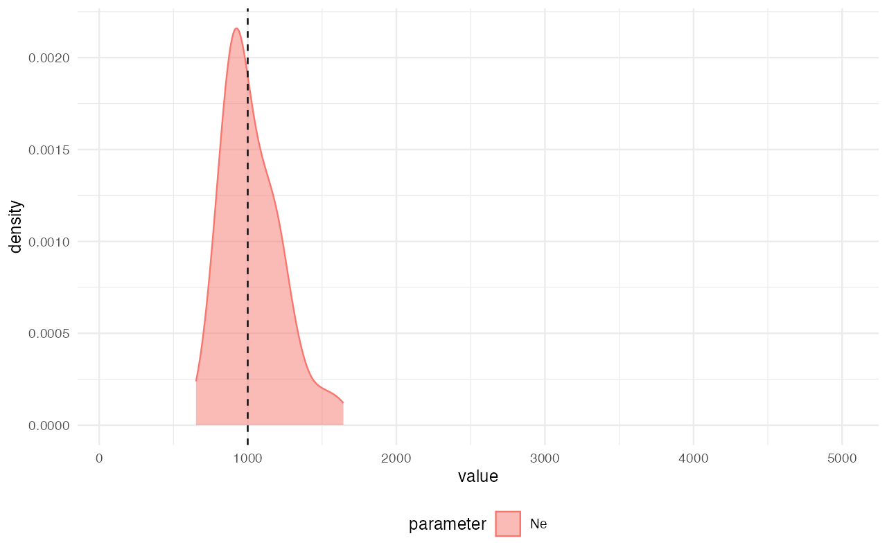
Because this observed diversity is based on simulated data
from a known model, we’ll indicate the true “hidden”
value with a vertical line.
extract_summary(abc)#> Warning in density.default(x, weights = weights): Selecting bandwidth *not*
#> using 'weights'#> Ne
#> Min.: 685.1383
#> Weighted 2.5 % Perc.: 730.6753
#> Weighted Median: 1008.6631
#> Weighted Mean: 1031.8771
#> Weighted Mode: 988.4247
#> Weighted 97.5 % Perc.: 1377.5585
#> Max.: 1519.6865
library(ggplot2)

plot_posterior(abc) +
  geom_vline(xintercept = 1000, linetype = "dashed") +
  coord_cartesian(xlim = c(100, 5000))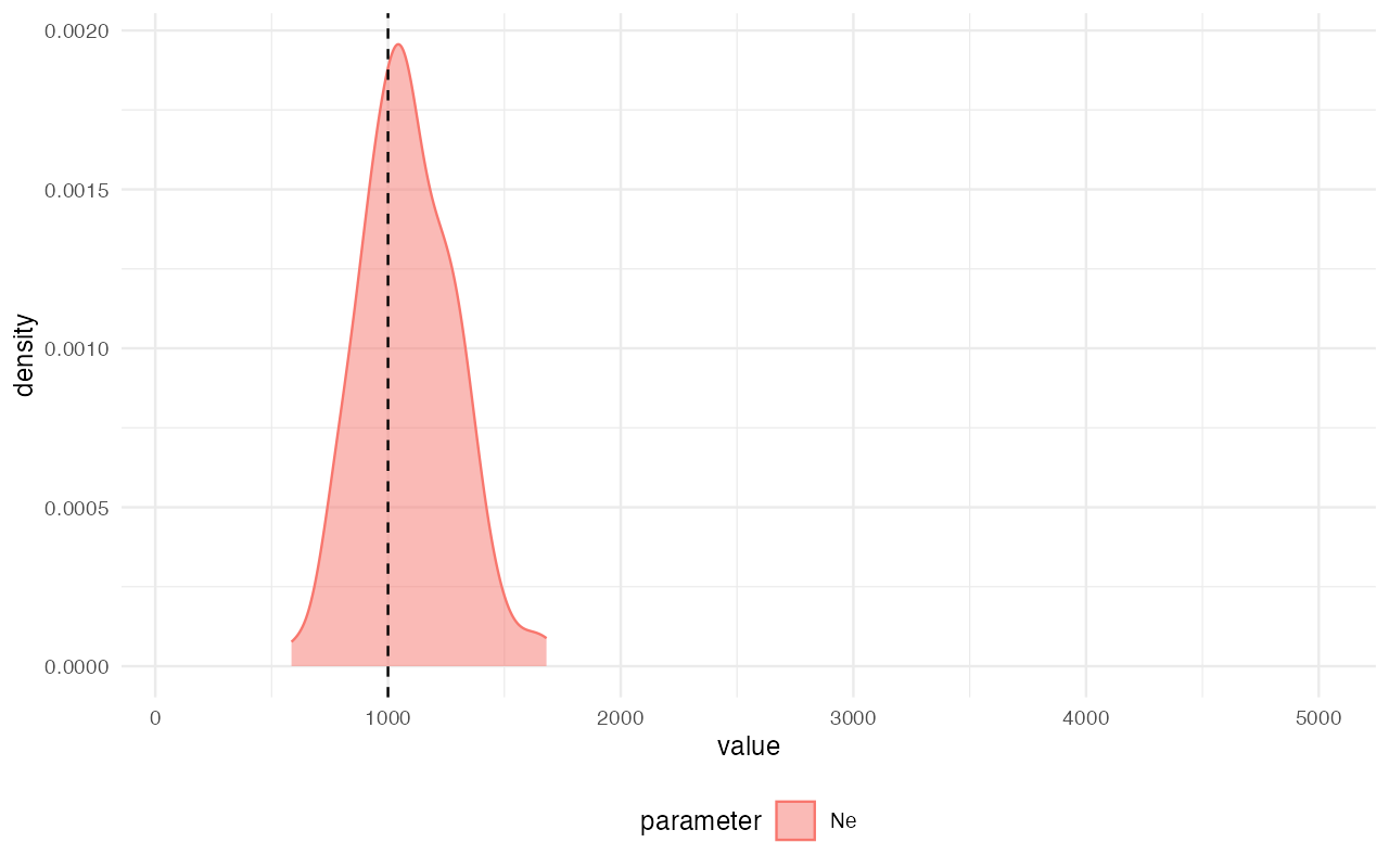
Using external programs to compute summary statistics
Now let’s move things one step forward. What if we either don’t find slendr’s tree-sequence interface to tskit sufficient and want to compute summary statistics from the simulated data using some external software, like PLINK or EIGENSTRAT?
To keep things as easy as possible (and avoid dragging in multiple
software dependencies), let’s say we have a program vcfpi,
which is run in the following way:
./vcfpi --vcf <path to a VCF> --tsv <path to a TSV table>You can find it at /private/var/folders/lq/bl36db_s6w908hnjkntdp4140000gn/T/RtmpWQy8Nd/temp_libpathec802a431124/demografr/examples/vcfpi) and run it yourself in the terminal.
This program takes in a VCF file and computes the nucleotide
diversity across all individuals in that VCF file. For simplicity, it
produces a table of results in exactly the same format as the
observed_diversity data frame above.
In this particular example, we want to replace the computation of
statistics performed by the R function compute_diversity in
the previous section (which also produces a data frame) with the product
of the external software vcfpi.
(We provide this vcfpi program as an example script, but
it could of course be any other program you could imagine.)
First, the definitions of priors and
observed statistics do not change:
# a single prior parameter
priors <- list(Ne ~ runif(100, 5000))

# a single observed statistic
observed <- list(diversity = observed_diversity)
What does change is the simulated summary statistics definition.
There are a number of ways we could go about this (and we will show
others below), but given that our vcfpi is a command-line
program, we will use the function
compute_pi_vcf <- function(vcf) {
  # path to the output summary statistic file
  tsv <- tempfile()

  # path to the example command-line utility (in this example we use a built-in toy program
  # called `vcfpi`, but this could be a path to any other program of your choosing, of course)
  program <- system.file("examples/vcfpi", package = "demografr")

  # execute the program on the command line using appropriate arguments
  system2(program, args = c("--vcf", vcf, "--tsv", tsv))

  # read the computed table with computed nucleotide diversity
  # (for simplicity, our example vcfpi program creates an output TSV
  # file already in the necessary format but any required reformatting
  # changes could easily happen at this stage)
  read.table(tsv, header = TRUE)
}

functions <- list(diversity = compute_pi_vcf)
There’s one last thing we need to do – our summary function
compute_diversity does not operate on a tree-sequence file
this time. Instead, vcfpi requires a VCF file as its input.
But, because of our simulation model python_script still
creates a tree-sequence file, we need to create a VCF to be able to
compute nucleotide diversity.
(Of course, we could modify the simulation model script to produce such VCF easily, but for the sake of making this example a bit more educational, let’s make our job a little bit harder).
Whenever we need to run a simulation summary statistic on a different
form of data than a tree-sequence, we can further customize the
data-generating function(s). In the first example, we had to provide a
function which creates a ts object from path
to a directory with all result files. In this example, let’s push this
one step further and create a VCF file.
(Again, we could’ve just as easily create a VCF file from our simulation script, but bear with me here!)
gens <- list(
  vcf = function(path) {
    # read the simulated tree sequence from a given path and subset it
    # (same code as previously, where we worked exclusively on tree sequences)
    ts_path <- file.path(path, "result.trees")
    ts <- ts_read(ts_path) %>% ts_simplify(simplify_to = seq(0, 99))

    # export genotypes from the tree sequence to a VCF (in the same directory)
    vcf_path <- file.path(path, "genotypes.vcf.gz")
    ts_vcf(ts, vcf_path)

    # return the path to the VCF for use in computing summary statistics
    return(vcf_path)
  }
)
model_run <- simulate_model(python_script, parameters = list(Ne = 123), format = "files", data = gens)When we look at the result, we can see that it no longer contains a
ts tree-sequence object but a path to a VCF file!
model_run#> $vcf
#> [1] "/private/var/folders/lq/bl36db_s6w908hnjkntdp4140000gn/T/RtmpUynJPfdemografr_1823336464/genotypes.vcf.gz"Let’s test our summary function on that VCF:
functions$diversity(model_run$vcf)#> set diversity
#> 1 pop 6.107462e-06Or, for convenience, we can do this using the more general function
summarise_data():
summarise_data(model_run, functions)#> $diversity
#>   set    diversity
#> 1 pop 6.107462e-06Now let’s validate our customized setup before we unleash the full scale of ABC simulations on the problem!
validate_abc(python_script, priors, functions, observed, data = gens, format = "files")#> ======================================================================
#> Testing sampling of each prior parameter:
#> - Ne ✅
#> ---------------------------------------------------------------------
#> The model is a custom user-defined msprime script
#> ---------------------------------------------------------------------
#> Simulating tree sequence from the given model... ✅
#> ---------------------------------------------------------------------
#> Validating custom data-generating functions... ✅
#> ---------------------------------------------------------------------
#> Generating data from simulation results:
#> - vcf (type character) ✅
#> ---------------------------------------------------------------------
#> Computing user-defined summary functions:
#> - diversity ✅
#> ---------------------------------------------------------------------
#> Checking the format of simulated summary statistics:
#> - diversity [data frame] ✅
#> ======================================================================
#> No issues have been found in the ABC setup!
library(future)
plan(multisession, workers = availableCores()) # parallelize across all CPUs

data <- simulate_abc(
  model = python_script, priors, functions, observed, iterations = 10000,
  data = gens, format = "files"
)
The total runtime for the ABC simulations was 0 hours 44 minutes 38 seconds parallelized across 96 CPUs.
Once the simulations are finished, we can perform inference of the posterior distribution of the single parameter of our model, :
abc <- run_abc(data, engine = "abc", tol = 0.01, method = "neuralnet")
extract_summary(abc)#> Warning in density.default(x, weights = weights): Selecting bandwidth *not*
#> using 'weights'#> Ne
#> Min.: 508.9297
#> Weighted 2.5 % Perc.: 583.1378
#> Weighted Median: 1027.3187
#> Weighted Mean: 1021.6676
#> Weighted Mode: 1004.5011
#> Weighted 97.5 % Perc.: 1432.5814
#> Max.: 1633.8342
library(ggplot2)

plot_posterior(abc) +
  geom_vline(xintercept = 1000, linetype = "dashed") +
  coord_cartesian(xlim = c(100, 5000))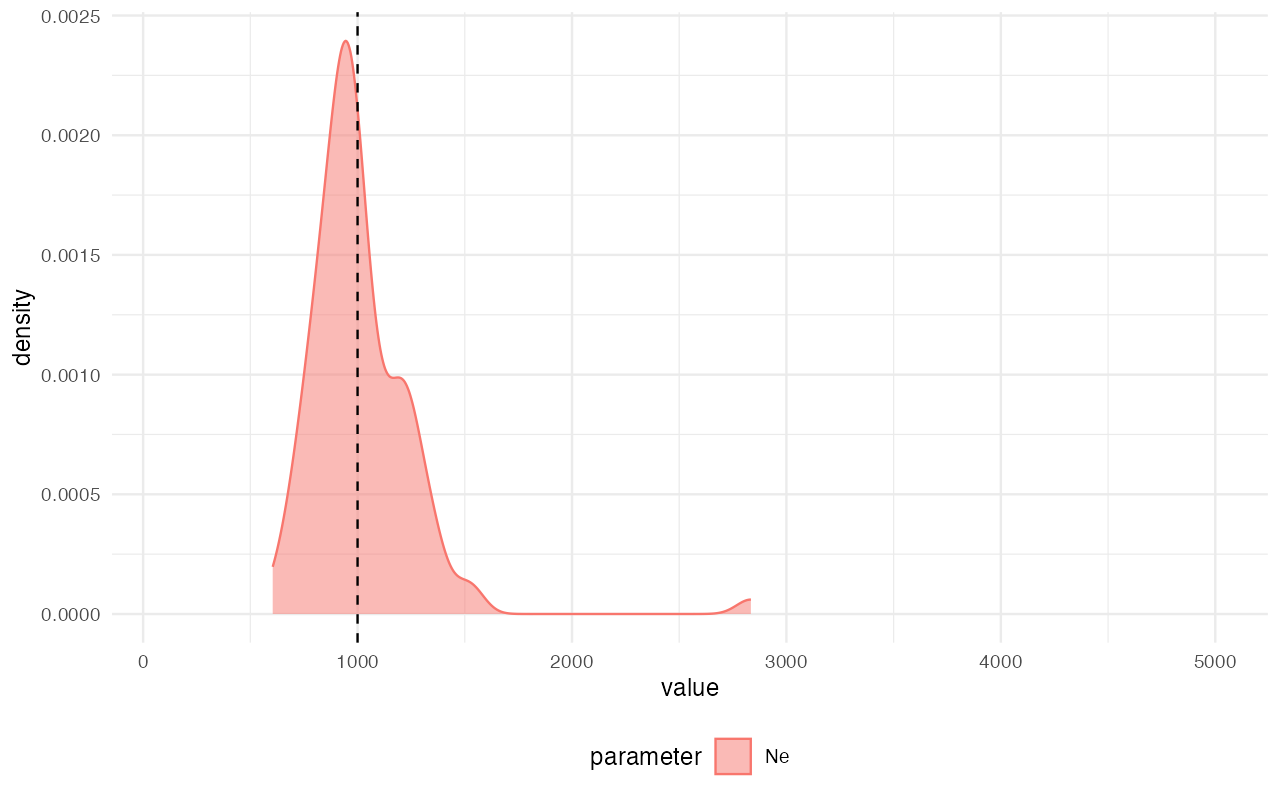
Another means of computing simulated summary statistics
Let’s look at a yet another variation of the same. What if we want to compute a summary statistics in R on a different source of genotype data (not a tree-sequence object in memory but also not a VCF file stored on disk)?
For instance, what if we want to compute a summary statistics on a
simple data frame of genotypes (0 – ancestral state,
1 – derived state).
We can modify our pipeline in the following way.
First, we need to define a summary statistic function which will
operate on a data frame, say called gt.
compute_diversity <- function(gt) {
  # generate a list of all pairs of chromosomes
  pairs <- combn(names(gt[, -1]), 2, simplify = FALSE)

  # count the number of nucleotide differences for each pair
  diffs <- sapply(pairs, function(pair) sum(gt[[pair[1]]] != gt[[pair[2]]]))

  # the mean is the nucleotide diversity of the sample of chromosomes
  pi <- mean(diffs) / 1e6

  data.frame(set = "pop", diversity = pi)
}

functions <- list(diversity = compute_diversity)
We also need a data-generating function, which will create the table of genotypes from standard simulated output:
gens <- list(
  gt = function(path) {
    # read the simulated tree sequence from a given path and subset it
    ts_path <- file.path(path, "result.trees")
    ts <- ts_read(ts_path) %>% ts_simplify(simplify_to = seq(0, 99))
    # suppress warnings due to multiallelic sites
    suppressWarnings(ts_genotypes(ts))
  }
)
And that’s it! Let’s check again that the whole setup works correctly.
model_run <- simulate_model(python_script, parameters = list(Ne = 123), format = "files", data = gens)When we look at the result, we can see that it no longer contains a
ts tree-sequence object but a simple table of genotypes
created via the slendr function ts_genotypes()
(see the data generating function just above).
model_run#> $gt
#> # A tibble: 19 × 101
#> pos pop_0_0_chr1 pop_0_0_chr2 pop_0_1_chr1 pop_0_1_chr2 pop_0_2_chr1
#> <int> <int> <int> <int> <int> <int>
#> 1 72887 1 0 0 0 0
#> 2 80420 0 0 0 0 1
#> 3 104320 0 0 0 0 1
#> 4 139183 0 0 0 0 0
#> 5 255690 1 0 1 0 0
#> 6 265572 1 0 1 1 0
#> 7 266899 0 0 0 0 0
#> 8 314855 0 0 0 0 0
#> 9 319324 0 0 0 0 0
#> 10 370142 1 0 1 0 0
#> 11 401629 0 0 1 0 0
#> 12 560741 0 1 0 0 1
#> 13 625599 0 0 0 0 0
#> 14 662845 1 0 0 0 0
#> 15 747451 0 0 0 0 1
#> 16 798418 0 0 0 0 0
#> 17 864122 0 0 0 0 0
#> 18 920561 1 0 1 0 0
#> 19 973502 0 0 0 1 0
#> # ℹ 95 more variables: pop_0_2_chr2 <int>, pop_0_3_chr1 <int>,
#> # pop_0_3_chr2 <int>, pop_0_4_chr1 <int>, pop_0_4_chr2 <int>,
#> # pop_0_5_chr1 <int>, pop_0_5_chr2 <int>, pop_0_6_chr1 <int>,
#> # pop_0_6_chr2 <int>, pop_0_7_chr1 <int>, pop_0_7_chr2 <int>,
#> # pop_0_8_chr1 <int>, pop_0_8_chr2 <int>, pop_0_9_chr1 <int>,
#> # pop_0_9_chr2 <int>, pop_0_10_chr1 <int>, pop_0_10_chr2 <int>,
#> # pop_0_11_chr1 <int>, pop_0_11_chr2 <int>, pop_0_12_chr1 <int>, …Let’s test our summary function on the output of the single testing simulation run:
summarise_data(model_run, functions)#> $diversity
#> set diversity
#> 1 pop 4.427475e-06Let’s also validate our customized setup before we unleash the full scale of ABC simulations on the problem!
validate_abc(python_script, priors, functions, observed, data = gens, format = "files")#> ======================================================================
#> Testing sampling of each prior parameter:
#> - Ne ✅
#> ---------------------------------------------------------------------
#> The model is a custom user-defined msprime script
#> ---------------------------------------------------------------------
#> Simulating tree sequence from the given model... ✅
#> ---------------------------------------------------------------------
#> Validating custom data-generating functions... ✅
#> ---------------------------------------------------------------------
#> Generating data from simulation results:
#> - gt (type tbl_df) ✅
#> ---------------------------------------------------------------------
#> Computing user-defined summary functions:
#> - diversity ✅
#> ---------------------------------------------------------------------
#> Checking the format of simulated summary statistics:
#> - diversity [data frame] ✅
#> ======================================================================
#> No issues have been found in the ABC setup!
library(future)
plan(multisession, workers = availableCores())

data <- simulate_abc(
  model = python_script, priors, functions, observed, iterations = 10000,
  data = gens, format = "files"
)
The total runtime for the ABC simulations was 0 hours 43 minutes 14 seconds parallelized across 96 CPUs.
Once the simulations are finished, we can perform inference of the posterior distribution of the single parameter of our model, :
abc <- run_abc(data, engine = "abc", tol = 0.01, method = "neuralnet")
extract_summary(abc)#> Warning in density.default(x, weights = weights): Selecting bandwidth *not*
#> using 'weights'#> Ne
#> Min.: 661.0598
#> Weighted 2.5 % Perc.: 670.1297
#> Weighted Median: 1023.4618
#> Weighted Mean: 1042.2674
#> Weighted Mode: 1008.6709
#> Weighted 97.5 % Perc.: 1445.8342
#> Max.: 1813.9612
library(ggplot2)

plot_posterior(abc) +
  geom_vline(xintercept = 1000, linetype = "dashed") +
  coord_cartesian(xlim = c(100, 5000))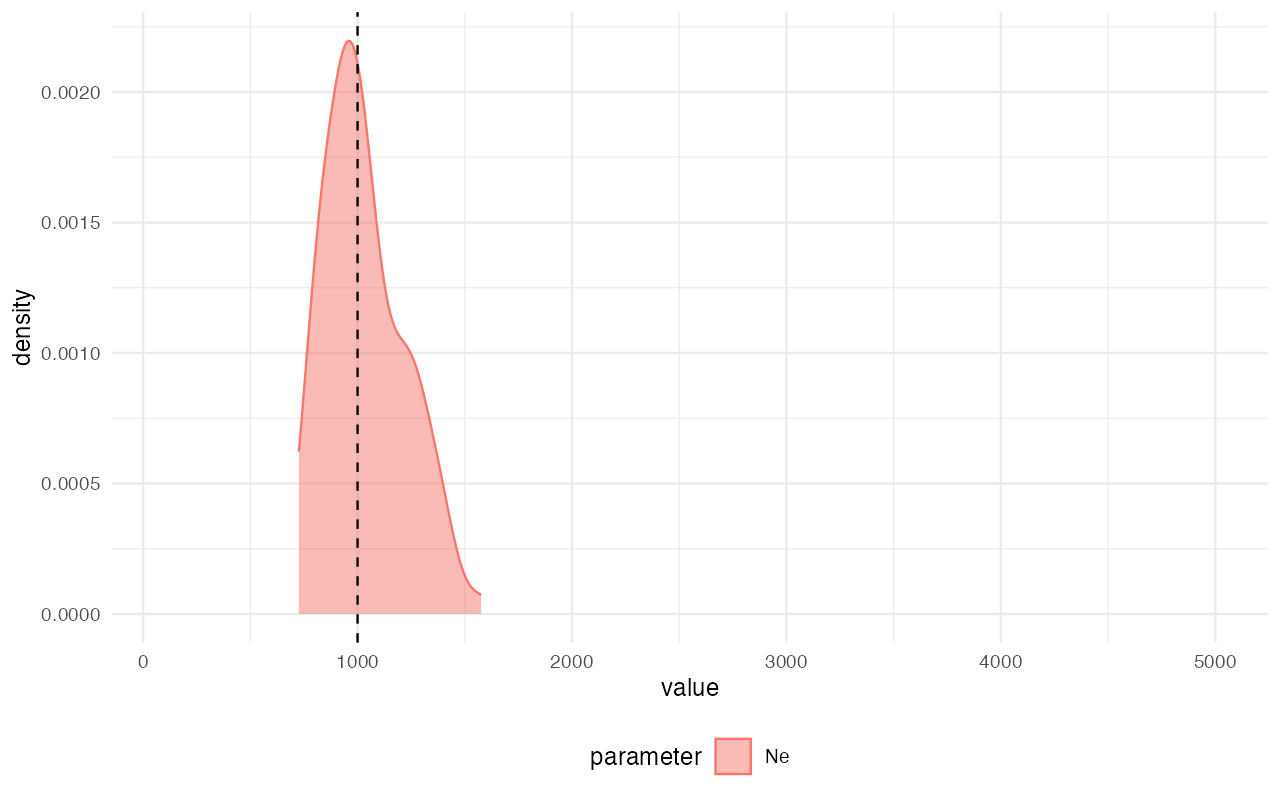
Computing summary statistics with Python
As a last example for customization of demografr inference pipeline, let’s consider the scenario in which the tree-sequence functionality available through slendr isn’t sufficient, and you need to compute summary statistics on the simulated tree-sequence using pure Python and the tskit module directly. As with the other customization examples above, this is again very easy to do.
First, just to change things up, let’s say that we want to use a normal slendr model function as a scaffold model for inference, simulate a tree sequence with the standard slendr / demografr functionality (i.e, not via the external Python script as in the examples above), and only customize the summary statistic computation of nucleotide diversity.
model <- function(Ne) {
  # this will be a single-population coalescent model, so the time of
  # the appearance of the population is arbitrary -- let's say we
  # want the model to start at 1000 generations ago, just to pick an
  # arbitrary point in time
  pop <- population("pop", N = Ne, time = 1000)
  model <- compile_model(
    pop, generation_time = 1,
    direction = "backward",
    serialize = FALSE
  )
  schedule <- schedule_sampling(model, times = 0, list(pop, 50))
  return(list(model, schedule))
}
We will use the same prior and observed statistic as above:
observed_diversity <- readRDS(get_cache("examples/custom_diversity.rds"))

priors <- list(Ne ~ runif(100, 5000))

observed <- list(diversity = observed_diversity)
compute_diversity <- function(ts) {
  reticulate::py_run_string(r"(
def compute_diversity(ts):
    diffs = []

    for i in range(ts.num_samples - 1):
        for j in range(i + 1, ts.num_samples):
            diffs.append(ts.divergence(sample_sets=[[i], [j]], mode="site"))

    pi = sum(diffs) / len(diffs)

    return pd.DataFrame({"set": ["pop"], "diversity": [pi]})
)"
  )
  reticulate::py$compute_diversity(ts)
}

functions <- list(diversity = compute_diversity)
model_run <- simulate_model(model, parameters = priors, sequence_length = 1e6, recombination_rate = 1e-8)When we look at the result, we can see that it no longer contains a
ts tree-sequence object but a simple table of genotypes
created via the slendr function ts_genotypes()
(see the data generating function just above).
model_run#> ╔═══════════════════════════╗
#> ║TreeSequence ║
#> ╠═══════════════╤═══════════╣
#> ║Trees │ 679║
#> ╟───────────────┼───────────╢
#> ║Sequence Length│ 1,000,000║
#> ╟───────────────┼───────────╢
#> ║Time Units │generations║
#> ╟───────────────┼───────────╢
#> ║Sample Nodes │ 100║
#> ╟───────────────┼───────────╢
#> ║Total Size │ 123.5 KiB║
#> ╚═══════════════╧═══════════╝
#> ╔═══════════╤═════╤═════════╤════════════╗
#> ║Table │Rows │Size │Has Metadata║
#> ╠═══════════╪═════╪═════════╪════════════╣
#> ║Edges │2,579│ 80.6 KiB│ No║
#> ╟───────────┼─────┼─────────┼────────────╢
#> ║Individuals│ 50│ 1.4 KiB│ No║
#> ╟───────────┼─────┼─────────┼────────────╢
#> ║Migrations │ 0│ 8 Bytes│ No║
#> ╟───────────┼─────┼─────────┼────────────╢
#> ║Mutations │ 0│ 16 Bytes│ No║
#> ╟───────────┼─────┼─────────┼────────────╢
#> ║Nodes │ 691│ 18.9 KiB│ No║
#> ╟───────────┼─────┼─────────┼────────────╢
#> ║Populations│ 1│222 Bytes│ Yes║
#> ╟───────────┼─────┼─────────┼────────────╢
#> ║Provenances│ 1│ 1.4 KiB│ No║
#> ╟───────────┼─────┼─────────┼────────────╢
#> ║Sites │ 0│ 16 Bytes│ No║
#> ╚═══════════╧═════╧═════════╧════════════╝Let’s test our summary function on the output of the single testing simulation run:
summarise_data(model_run, functions)#> $diversity
#> set diversity
#> 1 pop 0Let’s also validate our customized setup before we unleash the full scale of ABC simulations on the problem!
validate_abc(model, priors, functions, observed,
             sequence_length = 1e6, recombination_rate = 0)
#> ======================================================================
#> Testing sampling of each prior parameter:
#> - Ne ✅
#> ---------------------------------------------------------------------
#> The model is a slendr function
#> ---------------------------------------------------------------------
#> Checking the return statement of the model function... ✅
#> ---------------------------------------------------------------------
#> Checking the presence of required model function arguments...---------------------------------------------------------------------
#> Simulating tree sequence from the given model... ✅
#> ---------------------------------------------------------------------
#> Computing user-defined summary functions:
#> - diversity ✅
#> ---------------------------------------------------------------------
#> Checking the format of simulated summary statistics:
#> - diversity [data frame] ✅
#> ======================================================================
#> No issues have been found in the ABC setup!
library(future)
plan(multisession, workers = availableCores())

data <- simulate_abc(
  model, priors, functions, observed, iterations = 10000,
  sequence_length = 1e6, recombination_rate = 1e-8, mutation_rate = 1e-8
)
The total runtime for the ABC simulations was 0 hours 38 minutes 3 seconds parallelized across 96 CPUs.
Once the simulations are finished, we can perform inference of the posterior distribution of the single parameter of our model, :
abc <- run_abc(data, engine = "abc", tol = 0.01, method = "neuralnet")
extract_summary(abc)#> Warning in density.default(x, weights = weights): Selecting bandwidth *not*
#> using 'weights'#> Ne
#> Min.: 598.485
#> Weighted 2.5 % Perc.: 640.376
#> Weighted Median: 1007.319
#> Weighted Mean: 1014.007
#> Weighted Mode: 1080.402
#> Weighted 97.5 % Perc.: 1489.913
#> Max.: 1576.024
library(ggplot2)

plot_posterior(abc) +
  geom_vline(xintercept = 1000, linetype = "dashed") +
  coord_cartesian(xlim = c(100, 5000))