⚠️⚠️⚠️
Please note that until a peer reviewed publication describing the demografr package is published, the software should be regarded as experimental and potentially unstable.
⚠️️⚠️⚠️
This vignette contains an expanded version of the basic ABC inference example from the homepage of demografr. It walks through the process of setting up a demografr ABC inference pipeline step by step.
Introduction
Imagine that we sequenced genomes of individuals from populations “A”, “B”, “C”, and “D”.
Let’s also assume that we know that the populations are phylogenetically related in the following way but we don’t know anything else (i.e., we have no idea about the values of , split times, or gene-flow proportions):
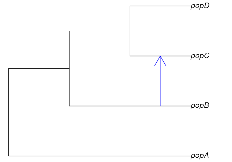
After sequencing the genomes of individuals from these populations, we computed nucleotide diversity in these populations as well as their pairwise genetic divergence and a one statistic, observing the following values of these summary statistics (which we saved in standard R data frames—perhaps saved by the software we used for computing these from empirical sequence data):
- Nucleotide diversity in each population:
observed_diversity <- read.table(system.file("examples/basics_diversity.tsv", package = "demografr"), header = TRUE)

observed_diversity
#> set diversity
#> 1 A 8.030512e-05
#> 2 B 3.288576e-05
#> 3 C 1.013804e-04
#> 4 D 8.910909e-05- Pairwise divergence d_X_Y between populations X and Y:
observed_divergence <- read.table(system.file("examples/basics_divergence.tsv", package = "demografr"), header = TRUE)

observed_divergence
#> x y divergence
#> 1 A B 0.0002378613
#> 2 A C 0.0002375761
#> 3 A D 0.0002379385
#> 4 B C 0.0001088217
#> 5 B D 0.0001157056
#> 6 C D 0.0001100633- Value of the following -statistic:
observed_f4  <- read.table(system.file("examples/basics_f4.tsv", package = "demografr"), header = TRUE)

observed_f4
#> W X Y Z f4
#> 1 A B C D -3.262146e-06Now let’s develop a simple ABC pipeline which will infer the posterior distributions of two sets of parameters we are interested in: of each population lineage, as well as split times between our populations of interest, and the gene-flow proportion.
Developing an ABC pipeline
Let’s begin by loading demografr together with the R package slendr on which demografr relies on for building and simulating demographic models.
library(demografr)
library(slendr)

# we also have to activate slendr's internal environment for tree sequences
# simulation and analysis
init_env()

# setup parallelization across all CPUs
library(future)
plan(multisession, workers = availableCores())
For the purpose of our ABC inference, we will bind all statistics in an R list, naming them appropriately. The names of each statistic (here “diversity”, “divergence”, and “f4”) have a meaning and are quite important for later steps:
observed <- list(
  diversity  = observed_diversity,
  divergence = observed_divergence,
  f4         = observed_f4
)
1. Setting up a “scaffold” model
The first step in a demografr ABC analysis is setting up a “scaffold” model—a slendr function which will produce a compiled slendr model object, and which will accept the model parameters in form of normal R function arguments. In our simple examples, we will define the following function:
model <- function(Ne_A, Ne_B, Ne_C, Ne_D, T_AB, T_BC, T_CD, gf_BC) {
  A <- population("A", time = 1,    N = Ne_A)
  B <- population("B", time = T_AB, N = Ne_B, parent = A)
  C <- population("C", time = T_BC, N = Ne_C, parent = B)
  D <- population("D", time = T_CD, N = Ne_D, parent = C)

  gf <- gene_flow(from = B, to = C, start = 9000, end = 9301, proportion = gf_BC)

  model <- compile_model(
    populations = list(A, B, C, D), gene_flow = gf,
    generation_time = 1, simulation_length = 10000,
    direction = "forward", serialize = FALSE
  )

  samples <- schedule_sampling(
    model, times = 10000,
    list(A, 25), list(B, 25), list(C, 25), list(D, 25),
    strict = TRUE
  )

  # when a specific sampling schedule is to be used, both model and samples
  # must be returned by the function
  return(list(model, samples))
}
2. Setting up priors
We are interested in estimating the of all populations, their split times, and gene-flow proportion which means we need to specify priors. demografr makes this very easy using its own readable syntax:
priors <- list(
  Ne_A  ~ runif(1000, 3000),
  Ne_B  ~ runif(100,  1500),
  Ne_C  ~ runif(5000, 10000),
  Ne_D  ~ runif(2000, 7000),

  T_AB  ~ runif(1,    4000),
  T_BC  ~ runif(3000, 9000),
  T_CD  ~ runif(5000, 10000),

  gf_BC ~ runif(0, 0.3)
)
In an ABC simulation step below, the formulas are used to draw the values of each parameter from specified distributions (in this case, all uniform distributions).
For more detail into how demografr’s prior sampling formulas work (and why), take a look at this vignette.
3. Defining summary statistics
Each run of a demografr ABC simulation internally produces a tree sequence. Because tree sequence represents an efficient, succint representation of the complete genealogical history of a set of samples, it is possible to compute population genetic statistics directly on the tree sequence without having to first save the outcome of each simulation to disk for computation in different software. Thanks to slendr’s library of tree-sequence functions serving as an R interface to the tskit module, we can specify summary statistics to be computed for ABC using normal R code.
In our example, because we computed nucleotide diversity, pairwise divergence, and from the sequence data, we will define the following summary statistic functions. Crucially, when run on a tree-sequence object, they will produce a data frame in the format analogous to the empirical statistics shown in data frames with the observed summary statistics above. This is a very important point: each observed statistic must have the same format (and dimension) as the data frames produced by the simulation summary functions. This minor inconvenience during ABC setup saves us the headache of having to match values of statistics between observed and simulated data during ABC inference itself.
compute_diversity <- function(ts) {
  samples <- ts_names(ts, split = "pop")
  ts_diversity(ts, sample_sets = samples)
}
compute_divergence <- function(ts) {
  samples <- ts_names(ts, split = "pop")
  ts_divergence(ts, sample_sets = samples)
}
compute_f4 <- function(ts) {
  samples <- ts_names(ts, split = "pop")
  A <- samples["A"]; B <- samples["B"]
  C <- samples["C"]; D <- samples["D"]
  ts_f4(ts, A, B, C, D)
}

functions <- list(
  diversity  = compute_diversity,
  divergence = compute_divergence,
  f4         = compute_f4
)
Of course, having to run ABC simulations in order to check that the
summary functions have been correctly defined would be slow and
potentially costly in terms of wasted computation. To speed this process
up, demografr provides a helper function
simulate_model() which allows us to simulate a single
tree-sequence object from the specified model. We can then use that tree
sequence to develop (and test) our summary functions before proceeding
further, like this:
ts <- simulate_model(model, priors, sequence_length = 1e6, recombination_rate = 1e-8)
ts
#> ╔═══════════════════════════╗
#> ║TreeSequence ║
#> ╠═══════════════╤═══════════╣
#> ║Trees │ 1,782║
#> ╟───────────────┼───────────╢
#> ║Sequence Length│ 1,000,000║
#> ╟───────────────┼───────────╢
#> ║Time Units │generations║
#> ╟───────────────┼───────────╢
#> ║Sample Nodes │ 200║
#> ╟───────────────┼───────────╢
#> ║Total Size │ 383.2 KiB║
#> ╚═══════════════╧═══════════╝
#> ╔═══════════╤═════╤═════════╤════════════╗
#> ║Table │Rows │Size │Has Metadata║
#> ╠═══════════╪═════╪═════════╪════════════╣
#> ║Edges │7,981│249.4 KiB│ No║
#> ╟───────────┼─────┼─────────┼────────────╢
#> ║Individuals│ 100│ 2.8 KiB│ No║
#> ╟───────────┼─────┼─────────┼────────────╢
#> ║Migrations │ 0│ 8 Bytes│ No║
#> ╟───────────┼─────┼─────────┼────────────╢
#> ║Mutations │ 0│ 16 Bytes│ No║
#> ╟───────────┼─────┼─────────┼────────────╢
#> ║Nodes │2,360│ 64.5 KiB│ No║
#> ╟───────────┼─────┼─────────┼────────────╢
#> ║Populations│ 4│331 Bytes│ Yes║
#> ╟───────────┼─────┼─────────┼────────────╢
#> ║Provenances│ 1│ 2.6 KiB│ No║
#> ╟───────────┼─────┼─────────┼────────────╢
#> ║Sites │ 0│ 16 Bytes│ No║
#> ╚═══════════╧═════╧═════════╧════════════╝With this ts object, we can, for instance, test that our
compute_f4 summary function is defined correctly (meaning
that it returns an
statistics table formatted in exactly the same way as the observed table
above):
functions$f4(ts)#> # A tibble: 1 × 5
#> W X Y Z f4
#> <chr> <chr> <chr> <chr> <dbl>
#> 1 A B C D 0Looks good! (We have zero
values because we didn’t specify mutation rate in
simulate_model, as we were only interested in the
compatibility of the formats and dimensions of both simulated and
observed
tables). Of course, in your pipeline, you might (should!) check that all
of your summary functions are set up correctly.
4. ABC simulations
Having defined the scaffold model, a set of priors for our parameters
of interest
(,
split times, gene-flow proportion), as well as two summary statistic
functions, we can integrate all this information into the function
simulate_abc().
Before we run a potentially computationally costly simulations, it is
a good idea to again validate the ABC components we have so far
assembled using the function validate_abc(). This provides
much more elaborate correctness checks beyond the simple testing of the
summary functions as we did above.
validate_abc(model, priors, functions, observed,
             sequence_length = 1e6, recombination_rate = 1e-8)
#> ======================================================================
#> Testing sampling of each prior parameter:
#> - Ne_A ✅
#> - Ne_B ✅
#> - Ne_C ✅
#> - Ne_D ✅
#> - T_AB ✅
#> - T_BC ✅
#> - T_CD ✅
#> - gf_BC ✅
#> ---------------------------------------------------------------------
#> The model is a slendr function
#> ---------------------------------------------------------------------
#> Checking the return statement of the model function... ✅
#> ---------------------------------------------------------------------
#> Checking the presence of required model function arguments...---------------------------------------------------------------------
#> Simulating tree sequence from the given model... ✅
#> ---------------------------------------------------------------------
#> Computing user-defined summary functions:
#> - diversity ✅
#> - divergence ✅
#> - f4 ✅
#> ---------------------------------------------------------------------
#> Checking the format of simulated summary statistics:
#> - diversity [data frame] ✅
#> - divergence [data frame] ✅
#> - f4 [data frame] ✅
#> ======================================================================
#> No issues have been found in the ABC setup!Having verified that all model components are set up correctly, we
can proceed to the ABC simulations themselves, using
demografr’s function simulate_abc():
data <- simulate_abc(
  model, priors, functions, observed, iterations = 10000,
  sequence_length = 10e6, recombination_rate = 1e-8, mutation_rate = 1e-8
)
The total runtime for the ABC simulations was 0 hours 30 minutes 55 seconds parallelized across 96 CPUs.
At this point we have generated summary statistics for simulations of models using parameters drawn from our priors. In the next step, we can finally do inference of our parameters.
5. ABC inference
Having all the information about observed and simulated data bound in
a single R object data, we can finally infer the posterior
distribution of our model parameters using ABC. demografr
includes a convenient function run_abc() which reformats
the simulated and observed data in a format required by the R package abc and
internally calls its own function abc().
Note that run_abc is just convenience wrapper around the
abc() function in the package
abc, saving us a lot of work with the reformatting of data that's otherwise necessary. As such, all parameters of the functionabc()can be provided torun_abc()`,
which will then pass them on appropriately.
abc <- run_abc(data, engine = "abc", tol = 0.01, method = "neuralnet")6. Posterior predictive check
Before we proceed with inferring values of the model parameters from their posterior distributions, we should check whether our model can actually produce summary statistics which match the statistics observed in the empirical data.
In order to do this, we can use demografr’s
predict() method which accepts two mandatory function
arguments: the first is the abc object generated by the
run_abc() function (containing, among other things, the
information about the inferred posteriors), and the number of draws to
take from the posterior distribution of the parameters:
# because we set up a parallelization plan() above, the predictions are
# computed in parallel across all available CPUs
predictions <- predict(abc, samples = 1000)
If we take a closer look at the produced result, we see that it’s a
data frame object with several special columns (so-called “list
columns”). Those columns contain nested data frames with the values
of tree-sequence summary statistics computed for each combination of the
parameter values. Because this data has the same format as the output of
the function simulate_grid() (in fact, internally it
is produced by this function), see the vignette on grid simulations for more detail how
to analyse this.
In order to examine the posterior predictive check results for
individual (or all) summary statistics, we can use the function
extract_prediction(). A convenient alternative to check the
results visually is provided by the function
plot_prediction(). For instance, we can take a look at the
distributions of divergences produced from the parameter posterior like
this:
plot_prediction(predictions, "diversity")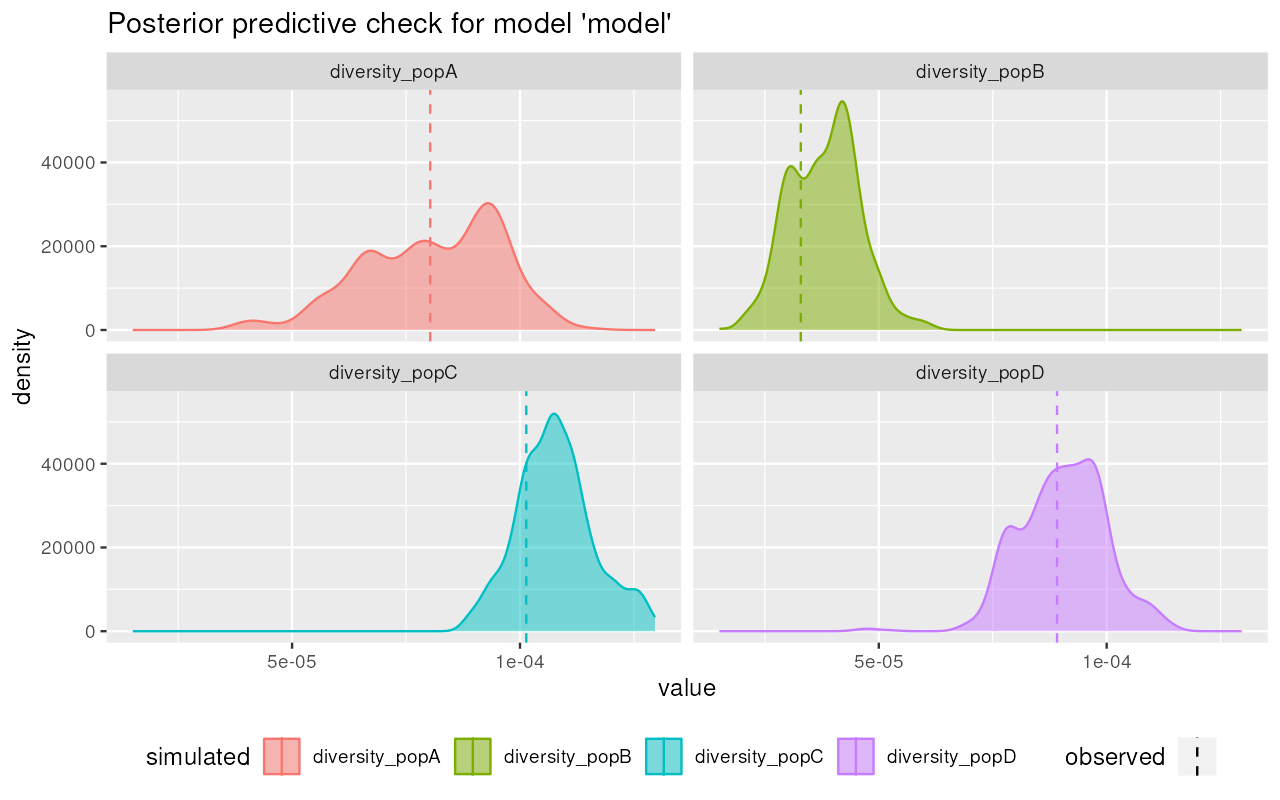
plot_prediction(predictions, "divergence")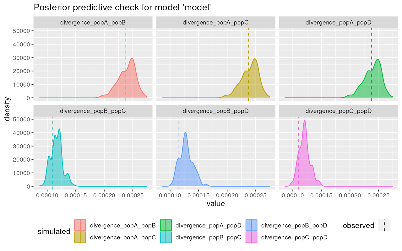
plot_prediction(predictions, "f4")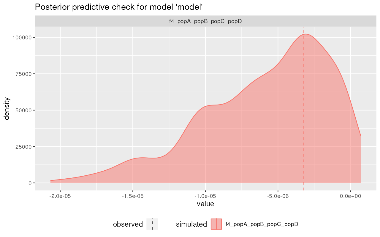
Nice! It appears that the posterior from our simplistic model captures the observed summary statistics (dashed vertical lines) quite well.
(To make evaluation a little bit easier, there’s an option
file = which instructs plot_prediction to save
a figure to disk instead of plotting it using a graphical device—useful
for work on remote servers!).
For more details on additional downstream validation and troubleshooting options, please see this vignette.
7. Extracting esimated parameters
Extracting posterior summary tables
Now that we have the ABC output object ready and have more or less convinced ourselves that our model can capture the summary statistics we’ve chosen via posterior predictive checks, we can proceed with parameter inference.
First, we can get a data frame with summary statistics of the posterior distributions of our parameters. For instance, we can easily read the maximum a posteriori probability (MAP) of the parameters in the row labelled “Mode:”:
extract_summary(abc)#> Ne_A Ne_B Ne_C Ne_D T_AB T_BC
#> Min.: 1492.557 526.6231 6373.061 2254.591 859.5749 5131.473
#> Weighted 2.5 % Perc.: 1774.758 672.5853 7344.040 2895.795 1318.3159 5595.637
#> Weighted Median: 2032.148 848.1467 8553.144 3814.660 1934.0008 6136.188
#> Weighted Mean: 2021.722 838.5594 8678.066 3804.614 1954.3343 6112.305
#> Weighted Mode: 2054.933 861.3408 8428.777 3721.917 1933.3694 6230.341
#> Weighted 97.5 % Perc.: 2270.334 1003.8421 10162.320 4530.273 2522.5919 6611.315
#> Max.: 2438.657 1047.0935 12703.479 5764.139 2650.7248 6851.800
#> T_CD gf_BC
#> Min.: 6752.669 -0.04681798
#> Weighted 2.5 % Perc.: 7125.349 0.02469992
#> Weighted Median: 7835.810 0.09867650
#> Weighted Mean: 7824.532 0.10282631
#> Weighted Mode: 7851.617 0.09804401
#> Weighted 97.5 % Perc.: 8426.377 0.18467366
#> Max.: 8476.157 0.21801675Because large tables can get a little hard to read, it is possible to subset to only a specific type of parameter:
extract_summary(abc, param = "Ne")#> Ne_A Ne_B Ne_C Ne_D
#> Min.: 1492.557 526.6231 6373.061 2254.591
#> Weighted 2.5 % Perc.: 1774.758 672.5853 7344.040 2895.795
#> Weighted Median: 2032.148 848.1467 8553.144 3814.660
#> Weighted Mean: 2021.722 838.5594 8678.066 3804.614
#> Weighted Mode: 2054.933 861.3408 8428.777 3721.917
#> Weighted 97.5 % Perc.: 2270.334 1003.8421 10162.320 4530.273
#> Max.: 2438.657 1047.0935 12703.479 5764.139
extract_summary(abc, param = "T")#> T_AB T_BC T_CD
#> Min.: 859.5749 5131.473 6752.669
#> Weighted 2.5 % Perc.: 1318.3159 5595.637 7125.349
#> Weighted Median: 1934.0008 6136.188 7835.810
#> Weighted Mean: 1954.3343 6112.305 7824.532
#> Weighted Mode: 1933.3694 6230.341 7851.617
#> Weighted 97.5 % Perc.: 2522.5919 6611.315 8426.377
#> Max.: 2650.7248 6851.800 8476.157Alternatively, we can also extract the posterior summary for a single model parameter like this:
extract_summary(abc, param = "gf_BC")#> gf_BC
#> Min.: -0.04681798
#> Weighted 2.5 % Perc.: 0.02469992
#> Weighted Median: 0.09867650
#> Weighted Mean: 0.10282631
#> Weighted Mode: 0.09804401
#> Weighted 97.5 % Perc.: 0.18467366
#> Max.: 0.21801675Visualizing posterior distributions of parameters
Because a chart is always more informative than a table, we can
easily get a visualization of our posteriors using the function
plot_posterior():
plot_posterior(abc, param = "Ne") + ggplot2::coord_cartesian(xlim = c(0, 10000))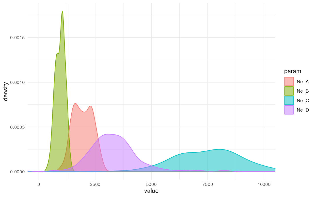
Excellent! It looks like we got really nice and informative posterior distributions of values!
Similarly, we get nice and informative posterior distributions of split times:
plot_posterior(abc, param = "T") + ggplot2::coord_cartesian(xlim = c(0, 10000))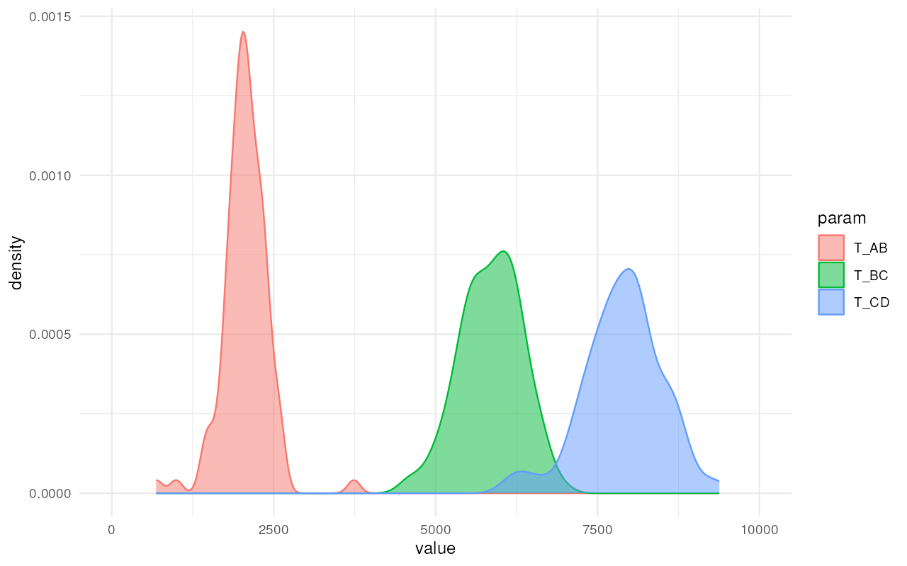
And the same is true for the gene-flow proportion:
plot_posterior(abc, param = "gf") + ggplot2::coord_cartesian(xlim = c(0, 1))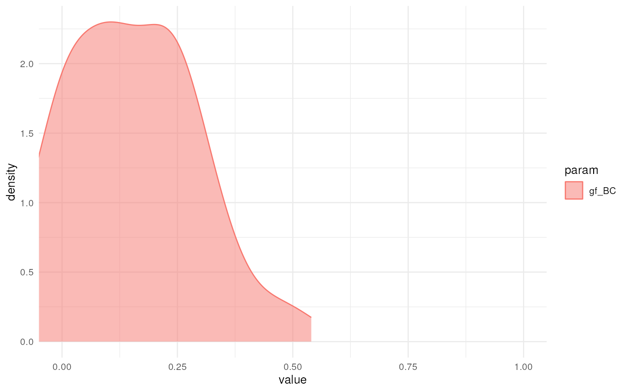
Because the internals of demografr ABC objects are represented by standard objects created by the abc package, we have all of the standard diagnostics functions of the abc R package at our disposal.
plot(abc, param = "T_BC")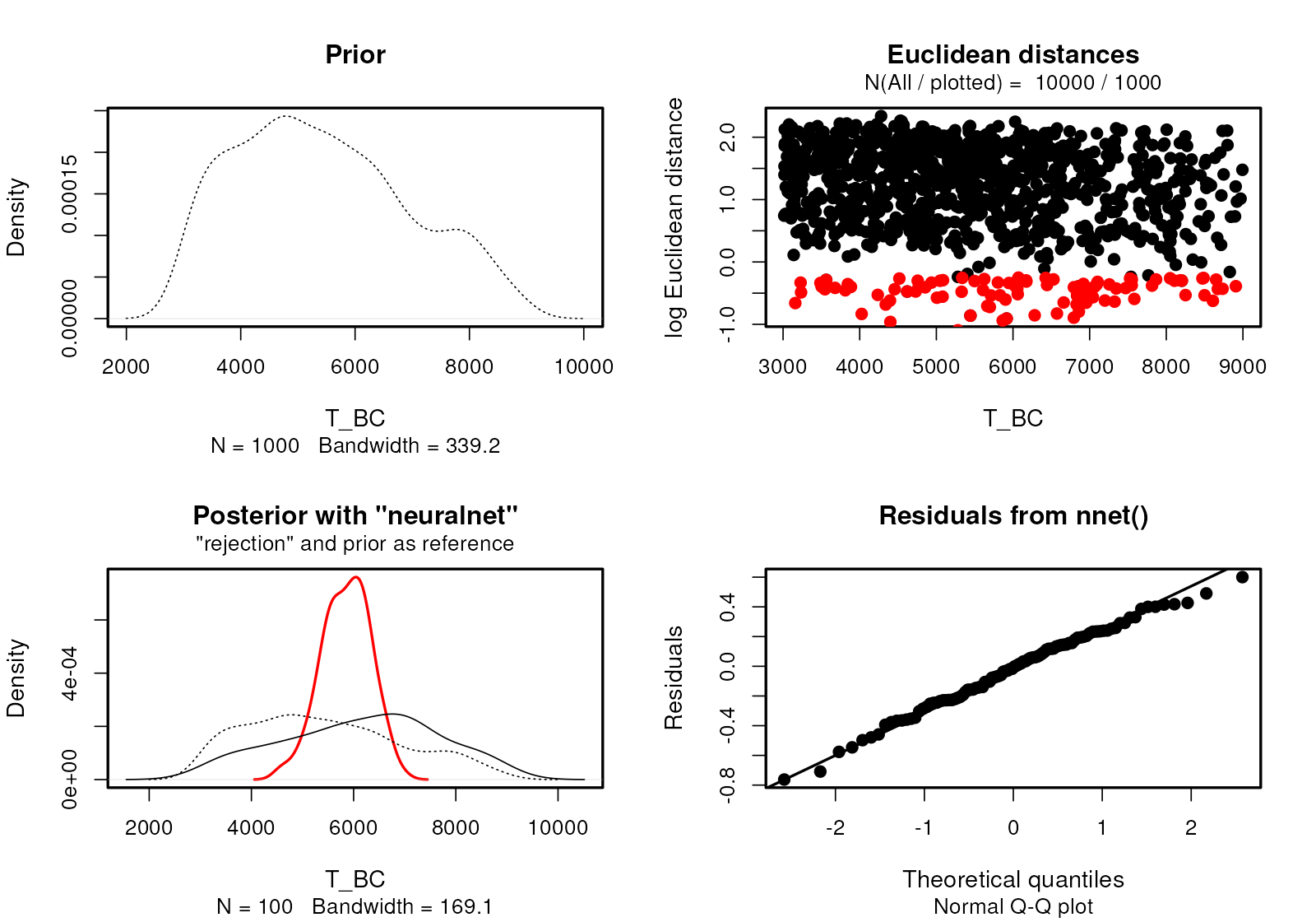
plot(abc, param = "gf_BC")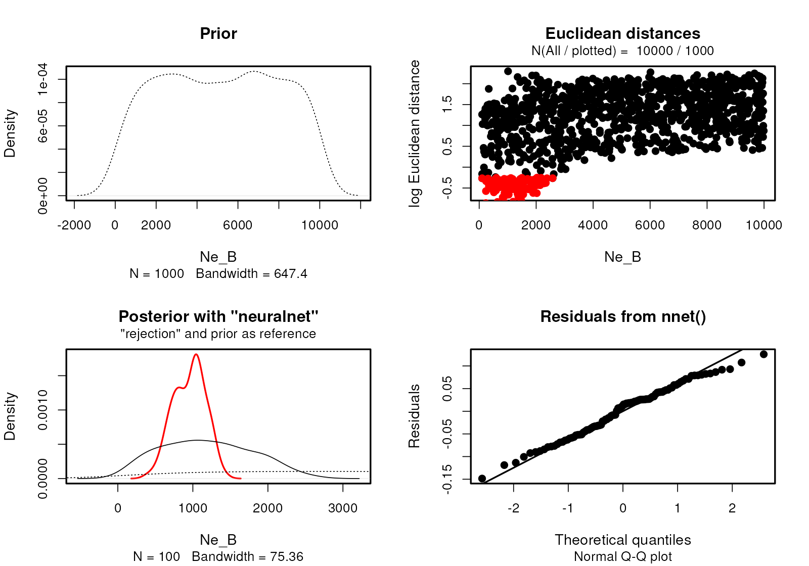
hist(abc, param = "Ne_D")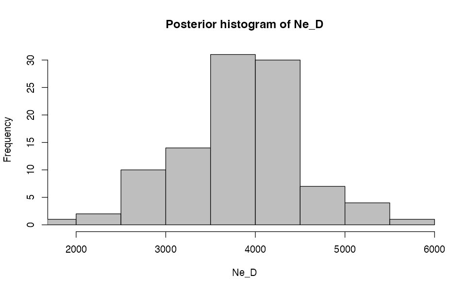
Again, there are numerous tools for additional diagnostics, which you can learn about here.