library(slendr)
init_env()

# build a basic population tree structure
p4 <- population("p4", time = 20000, N = 1000)
p3 <- population("p3", time = 6000, N = 1000, parent = p4)
p2 <- population("p2", time = 2000, N = 1000, parent = p3)
p1 <- population("p1", time = 1000, N = 1000, parent = p2)
px <- population("px", time = 500, N = 1000, parent = p2)

# compile the model and define recording of individuals
model <- compile_model(populations = list(p1, p2, p3, p4, px), generation_time = 1)
schedule <- schedule_recording(model, times = 0, list("each", 5))

# plot the model to check its correctness visually
plot_model(model, schedule = schedule)

# simulate 10 Mb of genomic data for later exploration
ts <-
  msprime(model, sequence_length = 10e6, recombination_rate = 1e-8, schedule = schedule) %>%
ts_mutate(mutation_rate = 1e-8)Tree thinking and \(f\) statistics
Theme of this chapter
In this chapter, we will delve a little bit into thinking about demographic histories (and about statistics we use to study those histories) through the lens of “tree thinking”—i.e., thinking in terms of genealogies recorded along the genome and, in particular, the branches in those genealogies. This fits the context of our work until this point quite naturally, particularly given the fact that the core component of slendr simulations is a tree sequence.
In the process, we will also change pace a bit, and use slendr as a sort of an “interactive popgen calculator” to quickly gain insights into population genetic statistics and explore them in an interactive way. Our main focus here will be on \(f\)-statistics and their interpretation through tracing paths along trees—particularly the \(f_4\) statistic—because they form such a crucial component of population genomics research.
Literature
If you want to know much more about the technical background of \(f_3\) and \(f_4\) statistics and admixture proportion estimators like \(f_4\)-ratio, you can take a look at the following papers: Peter, 2016, Lipson 2020, and Patterson et al., 2012.
There are a number of software tools that can compute various \(f\) statistics on real data. If you’d like to compare simulated \(f\) statistics to empirical results, take a look at ADMIXTOOLS 2 or my own R package admixr.
Exercise: “Outgroup” \(f_3\) as a measure of overlap of tree paths
To ease into the problem of interpreting \(f\)-statistics as measures of overlapping paths in “population trees” or—when admixture comes into the picture—in “admixture graphs”, let’s briefly return to our familiar \(f_3\) statistic.
Restart your R session, then create a new script f_null.R and paste the following code into that script. As always, read through the code, try to build a mental model of what it’s going to do, then run it and compare your understanding with the generated visualization of the model.
(I know this is easy, but being able to read code quickly and efficiently is the best way to learn to spot bugs.)
Now, consider the model implemented in our script f_null.R, visualized below:
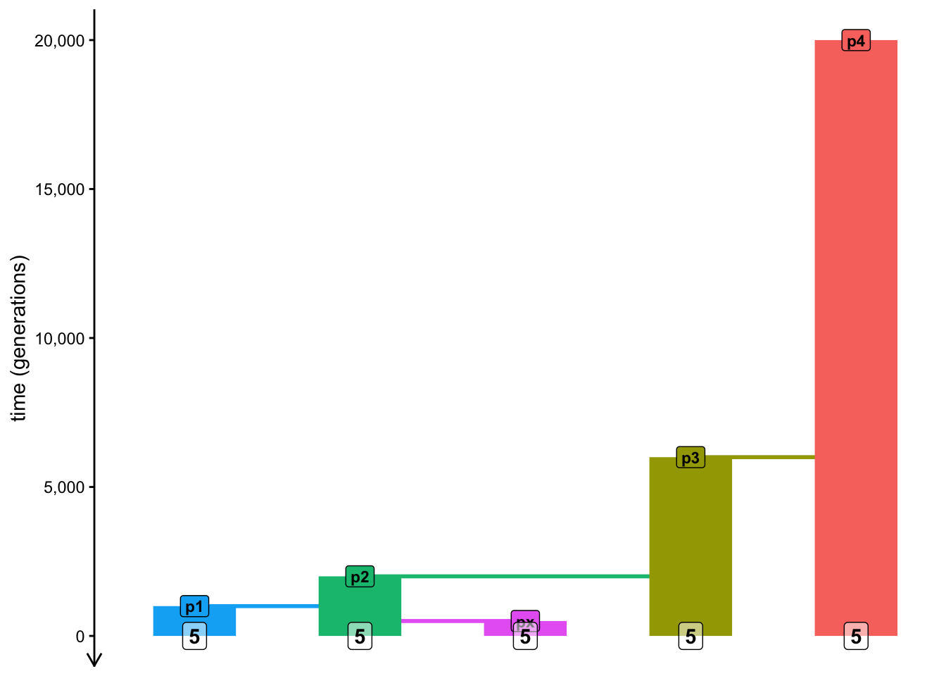
We know from the paper describing the theory of \(f\)-statistics and from our brief introduction that:
\(f_2(A, B)\) statistic measures the branch length between A and B (two individuals, two groups of individuals, two populations, etc.), and similarly
\(f_3(C; A, B)\) statistic is defined as the branch length which connects the internal most recent common ancestor node of A and B with the lineage C,
\(f_4\) (which we will discuss later) has a similar interpretation.
(These three ideas can be seen graphically in Figure 1 of that linked paper.)

Another thing established in the paper is the fact that any \(f\)-statistic can be expressed as a linear combination of multiple \(f_2\) statistics. In other words, you can “build” them by adding or subtracting multiple individual \(f_2\) branch lengths. If you’re not familiar with linear algebra, this might sound a bit obscure, but the idea is simple. More concretely, for instance, equation (20b) in the same paper states the following, which decomposes an \(f_3\) statistic into a composite of simpler \(f_2\) statistics (this is what “linear combination” basically is):
\[f_3(A; B, C) = \frac{1}{2} (f_2(A, C) + f_2(A, B) - f_2(B, C))\]
Draw a sketch of the population model (of populations p1, p2, p3, etc.) on a piece of paper, then trace by hand the paths indicated by the three \(f_2\) statistics in this equation on that sketch. When you “add” and “subtract” paths based on the equation (graphically by hand!), do you arrive at the definition of “outgroup” \(f_3\) as branch length from A and B towards the outgroup, as we described it in point 2. above?
When I was writing this chapter, I made a mistake in the equation above, which I discovered only after I wrote a quick simulation to double-check that the equation is correct. Let’s retrace my steps here because it shows why even very quick simulations can be really useful (almost like a “popgen calculator”!).
Let’s move to R. Use the function ts_f2() to implement this equation in code, computing a “homemade” \(f_3(A = p4; B = p1, C = p2)\) statistic which you just solved on paper, and compare it to the result you get if you run the computation using the ts_f3() function by slendr. Do you get the same result using both methods, and therefore verifying that the equation is correct?
Hint: You can either refer to entire populations in the ts_f2() like you did until now, or you can also use as A, B, and C single individuals (i.e., “pop4_1”, “pop1_1”, etc.).
Exercise: Mutations versus branches
Do you recall how I told you that you don’t have to add mutations to your tree sequence ts, and still be able to compute population genetic statistics? But that you can safely add them with ts_mutate() anyway?
The reason this works is because some very smart people figured out a mathematical duality between mutation-based and branch-based statistics—it actually doesn’t matter which way we compute our statistics, they give mathematically the same result in terms of theoretical statistical expectations (i.e., expectations of what happen in real data).
Repeat the previous exercise, but this time specify mode = "branch" in all your ts_f3() and ts_f2() commands. I suggest that you make a copy of your ts_f3() and ts_f2()-based code in your f_null.R script and and modify the copies for easier comparison of the results. What numbers do you get compared to the results of the previous exercise in terms of their scale? Can you relate those values to what your population tree model visualization indicates (in terms of branch lengths)? Look at your sketch with pen and paper again if this helps in putting your results in clearer context (particularly with regards to split times).
NoteClick to see the solution
Here are the two code chunks from the previous solution computed by setting mode = "branch":
ts_f3(ts, A = s["p4"], B = s["p1"], C = s["p2"], mode = "branch")# A tibble: 1 × 5
A B C statistic f3
<chr> <chr> <chr> <chr> <dbl>
1 p4 p1 p2 f3(p4;p1,p2) 11037.homemade_f3 <- (
ts_f2(ts, A = s["p4"], B = s["p1"], mode = "branch")$f2 +
ts_f2(ts, A = s["p4"], B = s["p2"], mode = "branch")$f2 -
ts_f2(ts, A = s["p1"], B = s["p2"], mode = "branch")$f2
) / 2
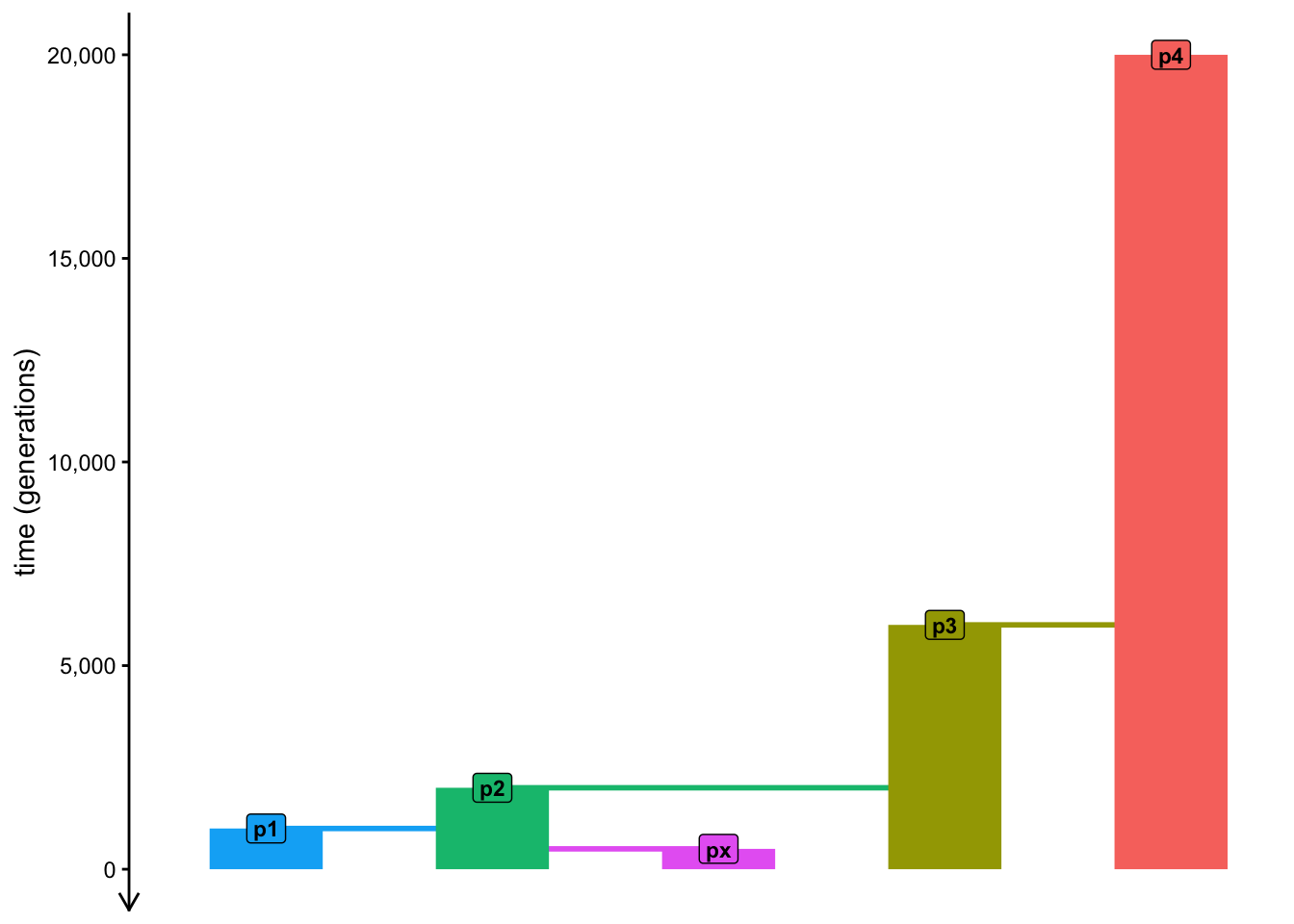
homemade_f3[1] 11036.96We can see that when we specify mode = "branch", the returned values of \(f\) statistics correspond to the real branch lengths in terms of times in generations! To see this, just take a look at your model sketch again, counting how much time there’s between split times. This is quite cool because as we discussed, the mathematical expectation of \(f_3\) statistic does, in fact, represent the overlap of paths in a tree going from p1 and p2 to the outgroup p4:
Hopefully, you can now appreciate that there’s nothing magical about \(f\) statistics. Even though their practical interpretation can get sometimes complicated, internally they always boil down to tracing paths through population trees in order to obtain statistical expectations of allele frequency correlations between lineages under study (interpreted as branch lengths), easily visualized by tracing paths through population trees.
In a way, setting mode = "branch" can be understood as instructing slendr to compute the results — in this case, of the \(f_3\) statistic — in “real time units” (in the case of this simple model, in generations).
Exercise: Basic intuition into the \(f_4\) statistic
Now let’s finally dig into exploring the most critical component of population genetics research (particularly in the context of ancient DNA)—the venerable \(f_4\)-statistic, formally established by Nick Patterson and David Reich in 2012.
From the intuitive follow-up paper on \(f\)-statistics by Benjamin Peter, we know that (in a very similar way to \(f_2\) and \(f_3\)) the \(f_4(W, X; Y, Z)\) statistic can be interpreted as the overlap between the paths in a tree connecting the pairs W-X and Y-Z, as is demonstrated in Figure 1 of the linked paper.
That said, what value does any given \(f_4\) statistic actually gives you depends on the (in practice, hidden) underlying demographic model which determines how populations are related—this is what we need to infer—and also what individuals assign into each of the four positions of the \(f_4\) “quartet configuration”.
Knowing the relationships between populations encoded by the tree model programmed in your script f_null.R and the interpretation of the \(f_4\) statistic, what is the expected value of \(f_4(p1, px; p3, p4)\) for this model? Try to answer by taking a look at the sketch of your model and tracing the path overlaps between p1-px and p3-p4 pairs, then compute the statistic on a ts simulated data with the ts_f4() function to verify your intuition. Does your simulation give you the exact result you might expect based on the visualization of the model alone? If it doesn’t give you the exact expected result, why could this be?
As suggested in the solution above, the reason we don’t get a perfectly zero expected value of the \(f_4\) is because of ILS and stochasticity. Let’s test this hypothesis now.
First, evaluate ts in your R console and note how many trees do you have in your 10 Mb tree-sequence.
Now, restart your R session (Session -> Restart R). Then, temporarily change the N of all populations in your model to 1 and re-run your script to get a new ts and compute the same \(f_4\) statistic again. \(N_e = 1\) implies a ludicrously high amount of drift, which should eliminate ILS completely, giving us \(f_4\) close to its mathematical expectation of zero. Is this true in your new simulation? And how many trees does your tree sequence have with this high amount of drift?
Of course, changing \(N_e\) to value of 1 as we did above is a drastic measure of only theoretical utility. We could hardly get away with doing that, if we wanted to use simulations to make a point in our research paper.
How do we deal with the unavoidable stochasticity in our simulations then? This wasn’t much of a problem in exercises in the previous chapters, but we need the way to solve this to be able to get useful, applicable results.
Let’s look into this now.
Exercise: Reducing stochastic noise via simulation replicates
First, set the N sizes of your populations in your model from 1 back to 1000, then re-run your script to make sure the original model is compiled (ideally by restarting R again).
As a means to tame the stochasticity and help meaningful statistical patterns stand out, I recently implemented a new slendr function ts_replicate(), specifically for this workshop! The way it works is like this:
ts_replicate(
  n = <number of replicates to simulate>,
  {
    # ...
    # a block of slendr code wrapped in { ... } containing a ts simulation
    # and a statistical computation we want to run in given replicates
    # ...
  }
)
Take a look at its manual page under ?ts_replicate, then use it to run 10 replicate simulations of the \(f_4\) statistic above (the one which should give us exactly zero value, but didn’t), saving the result to variable df. What format does the result have? When you visualize the distribution of \(f_4\) values across all 10 replicates, are they more interpretable in terms of the statistical expectation for this particular \(f_4\) “quartet”?
Note: If you want to speed up the replicate simulation, note that ?ts_replicate allows running multiple simulations in parallel.
NoteClick to see the solution
Here’s how we can modify the “template” above to answer this question:
df <- ts_replicate(

  # run 10 replicates ...
  n = 10,

  # ... of the following block of code...
  {

  # ... which first simulates a tree sequence ...
  ts <-
    msprime(model, sequence_length = 10e6, recombination_rate = 1e-8, schedule = schedule) %>%
    ts_mutate(mutation_rate = 1e-8)

  # ... and then computes a data frame with the given f4 statistic ...
  s <- ts_names(ts, split = TRUE)
  ts_f4(ts, W = s["p1"], X = s["px"], Y = s["p3"], Z = s["p4"])

  } # ... the function automatically binds all data frames into single one
)
We can see that we get the same format of the data frame as normally produced by the ts_f4() function, except with a new column rep added, indicating a replicate number.
df# A tibble: 10 × 7
W X Y Z statistic f4 rep
<chr> <chr> <chr> <chr> <chr> <dbl> <int>
1 p1 px p3 p4 f4(p1,px;p3,p4) -0.000000229 1
2 p1 px p3 p4 f4(p1,px;p3,p4) 0.000000476 2
3 p1 px p3 p4 f4(p1,px;p3,p4) -0.00000104 3
4 p1 px p3 p4 f4(p1,px;p3,p4) 0.000000852 4
5 p1 px p3 p4 f4(p1,px;p3,p4) 0.000000765 5
6 p1 px p3 p4 f4(p1,px;p3,p4) 0.000000452 6
7 p1 px p3 p4 f4(p1,px;p3,p4) 0.000000278 7
8 p1 px p3 p4 f4(p1,px;p3,p4) 0.00000111 8
9 p1 px p3 p4 f4(p1,px;p3,p4) 0.0000000240 9
10 p1 px p3 p4 f4(p1,px;p3,p4) -0.000000128 10This means we can visualize their distribution easily like this, for example:
library(ggplot2)

ggplot(df, aes(statistic, f4)) +
  geom_boxplot() +
  geom_jitter() +
  geom_hline(yintercept = 0, color = "red", linetype = "dashed")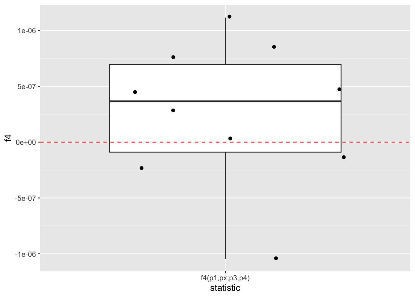
As we can see, when we run multiple replicates of the simulation, we are able to “control” the stochastic noise a bit, making the expected pattern stand out more clearly: we see that the expected value of f4(p1,px;p3,p4) is really zero (up to that unavoidable stochastic noise shown by the scatter of individual replicate values around zero).
Exercise: Other \(f_4\) “quartets”
Of course, \(f_4(p1, px; p3, p4)\) is only one possible “quartet configuration”.
Expand your 10 replicates simulation \(f_4(p1, px; p3, p4)\) by adding the computation of \(f_4(p1, p3; px, p4)\) and \(f_4(p1, p4; px, p3)\) in the same { ... } block provided to ts_replicate() (making sure you rbind() all three data resulting frames together at the end of the { ... } block).
How would you compare the interpretation of the three \(f_4\) statistics against one another? Again, use sketching of paths on a population tree on paper to try to figure it out first based on the definition of what \(f_4\) between the given two pairs of lineages indicate, then compare your understanding to what you see when you visualize the distributions of those three statistics.
Hint: This requires some ggplot2 visualization knowledge. Feel free to take a peek at my solution to learn how to plot the results, or just my own visualization for interpreting the differences between the three statistics.
NoteClick to see the solution
Let’s add the computation of all three \(f_4\) statistics in the same replicate simulation pipeline:
df <- ts_replicate(
  n = 10, {
  ts <-
    msprime(model, sequence_length = 10e6, recombination_rate = 1e-8, schedule = schedule) %>%
    ts_mutate(mutation_rate = 1e-8)

  s <- ts_names(ts, split = TRUE)

  # instead of computing one f4 like before, we compute all three and then
  # bind the three data frames into a single one
  rbind(
    ts_f4(ts, W = s["p1"], X = s["px"], Y = s["p3"], Z = s["p4"]), # 1st f4
    ts_f4(ts, W = s["p1"], X = s["p3"], Y = s["px"], Z = s["p4"]), # 2nd f4
    ts_f4(ts, W = s["p1"], X = s["p4"], Y = s["px"], Z = s["p3"])  # 3rd f4
  )
})
Again, we get a data frame with multiple replicates for each of the three statistics:
df# A tibble: 30 × 7
W X Y Z statistic f4 rep
<chr> <chr> <chr> <chr> <chr> <dbl> <int>
1 p1 px p3 p4 f4(p1,px;p3,p4) 0.00000197 1
2 p1 p3 px p4 f4(p1,p3;px,p4) 0.00000958 1
3 p1 p4 px p3 f4(p1,p4;px,p3) 0.00000761 1
4 p1 px p3 p4 f4(p1,px;p3,p4) 0.00000278 2
5 p1 p3 px p4 f4(p1,p3;px,p4) 0.00000783 2
6 p1 p4 px p3 f4(p1,p4;px,p3) 0.00000506 2
7 p1 px p3 p4 f4(p1,px;p3,p4) -0.000000366 3
8 p1 p3 px p4 f4(p1,p3;px,p4) 0.00000957 3
9 p1 p4 px p3 f4(p1,p4;px,p3) 0.00000994 3
10 p1 px p3 p4 f4(p1,px;p3,p4) -0.000000848 4
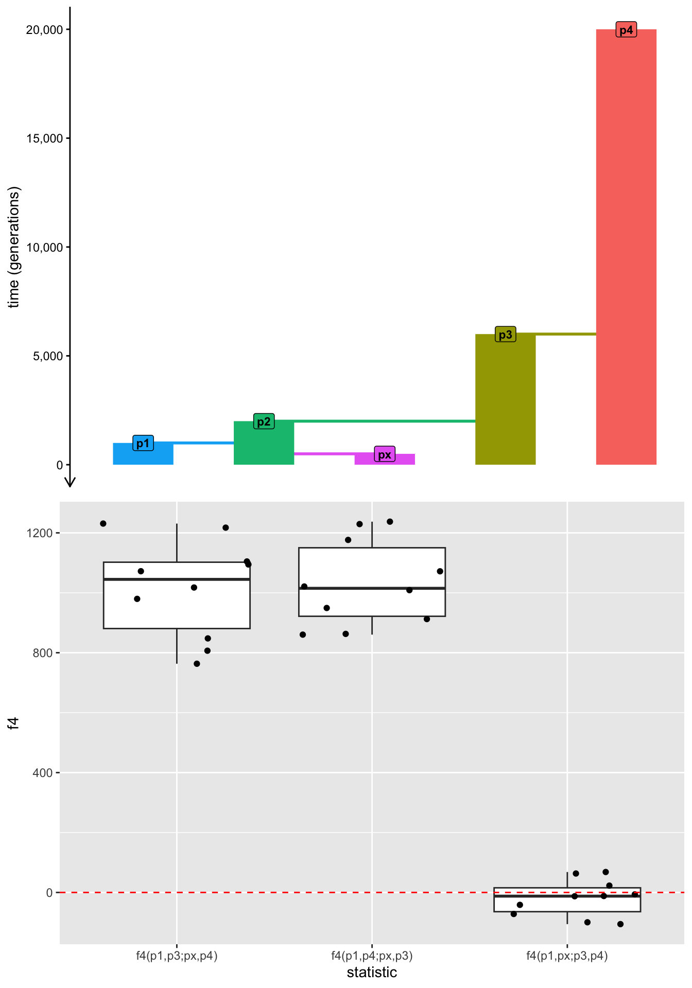
# ℹ 20 more rowsFrom the mathematical definition of \(f_4\) as internal branch lengths between two pairs of lineages in a given “quartet” and knowing the topological structure of our population tree, we can predict that the first \(f_4\) is expected to be zero (which is what we established earlier), and the other two \(f_4\) statistics are expected to have the same value representing the internal branch length connecting two pairs in the “quartet”.
This is exactly what we see in our results:
ggplot(df, aes(statistic, f4)) +
  geom_boxplot() +
  geom_jitter() +
  geom_hline(yintercept = 0, color = "red", linetype = "dashed")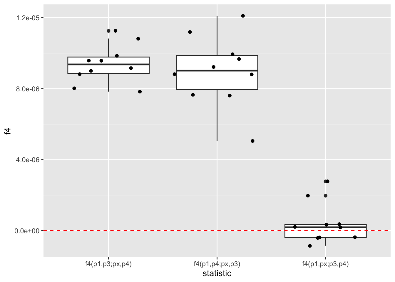
Make a copy of your ts_replicate() code computing the three \(f_4\) statistics and modify it by setting mode = "branch", as we did before, perhaps changing df to df_branch in this copied code for easier comparison. Recall that mode = "branch" instructs slendr’s internal statistical machinery to use “model time units” (here, generations) in computing the results based on branches, instead of mutations. When you visualize the three \(f_4\) statistics computed in this way, do you see this being reflected in the scale (and meaning) of the numbers which you get back?
NoteClick to see the solution
Let’s save the result in a new data frame df_branch:
df_branch <- ts_replicate(
  n = 10, {
  ts <-
    msprime(model, sequence_length = 10e6, recombination_rate = 1e-8, schedule = schedule) %>%
    ts_mutate(mutation_rate = 1e-8)

  s <- ts_names(ts, split = TRUE)

  rbind(
    ts_f4(ts, W = s["p1"], X = s["px"], Y = s["p3"], Z = s["p4"], mode = "branch"), # 1st f4
    ts_f4(ts, W = s["p1"], X = s["p3"], Y = s["px"], Z = s["p4"], mode = "branch"), # 2nd f4
    ts_f4(ts, W = s["p1"], X = s["p4"], Y = s["px"], Z = s["p3"], mode = "branch")  # 3rd f4
  )
})
When we visualize the results, we do indeed see that the f4 column contains the expected branch lengths expressed in real generation times! Here are the results plotted alongside the model using the package cowplot so that the branch length times can be read more easily:
library(cowplot) # get access to the plot_grid() function

plot_grid(
  # first panel:
  plot_model(model),

  # second panel:
  ggplot(df_branch, aes(statistic, f4)) +
    geom_boxplot() +
    geom_jitter() +
    geom_hline(yintercept = 0, color = "red", linetype = "dashed"),

  # plot both panels in two rows:
  nrow = 2
)
Catching up
This was a lot of work! If you want to check in with the state of our \(f\)-statistics exploratory simulation script f_null.R, here it is in the form which showcases the most important results from this chapter so far:
Exercise: Interpreting \(f_4\) as an admixture hypothesis test
Admittedly, thinking about \(f\) statistics as measures of allele frequency correlations between populations and interpreting them as overlapping branch lengths is intellectually interesting in terms of population genetics theory, but in practice, they are most famous (and most famously used) as admixture tests.
Create a new script f_admixture.R and copy my solutions to the exercises in this chapter available under the “Catching up” section above into that script. This is just to get the same starting point. Restart your R session (Session -> Restart R) then skim through this script and re-run it. Having gone through the exercises, the code should look somewhat familiar and the visualization you obtain by typing out p_panels into your R console (the branch lengths encoded by the three \(f_4\) statistics we studied) should make sense.
NoteClick to see the solution
Here’s the final visualization of the three \(f_4\) statistics for easier reference as you work on the following exercise.
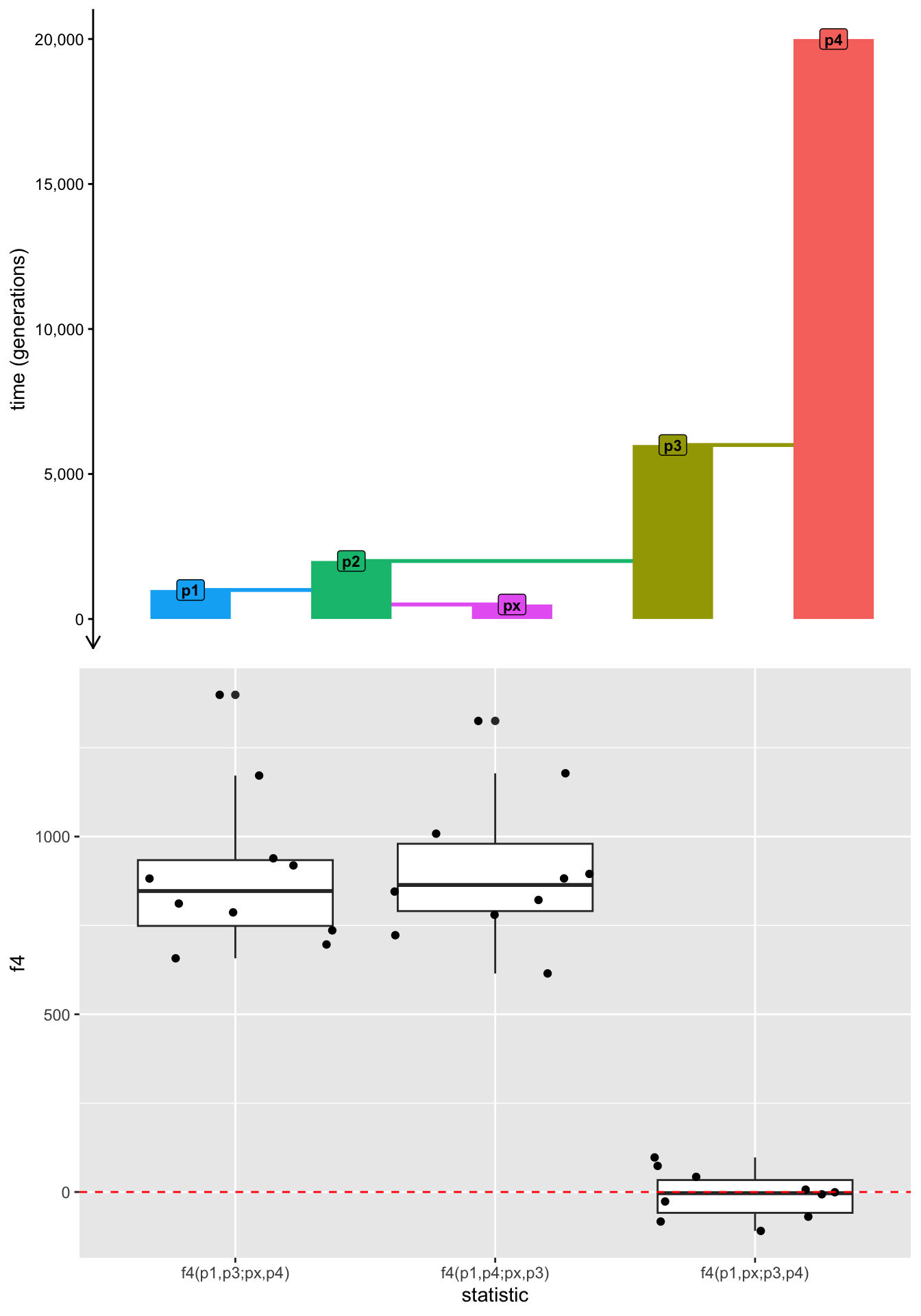
Right now our script f_admixture.R doesn’t have any admixture. It still contains what we established in this chapter so far: a statistical null model of “nothing interesting happened in the demographic history in terms of potential admixture”, as is reflected in the \(f_4\) values we obtained–most importantly in the “null hypothesis” statistic \(f_4(p1,px;p3,p4)\) being zero.
Introduce the following two changes to the f_admixture.R script to turn it into an admixture model:
Program a
gene_flow()eventgf, introducing 20% gene-flow fromp3topxbetween 400 and 300 generations ago.Add this
gfevent into themodelcompilation step executed bycompile_model().
With the steps 1. and 2. done, your model now includes admixture. Re-run the script again, and inspect the final visualization obtained by typing out p_panels into your R console. You should see an admixture edge added to your population tree.
How does admixture from p3 to px affect the branch lengths compared to the previous model f_null.R when you visualize the replicates for each of the three \(f_4\) statistics from the admixture model? Pay particular attention to the \(f_4(p1,px;p3,p4)\) statistic which had an expected value of zero before—does it still have a zero value? If not, why, and what does it tell us about it utility to study admixture histories?
NoteClick to see the solution
Here’s only the final visualization of the figure in the p_panel variable:
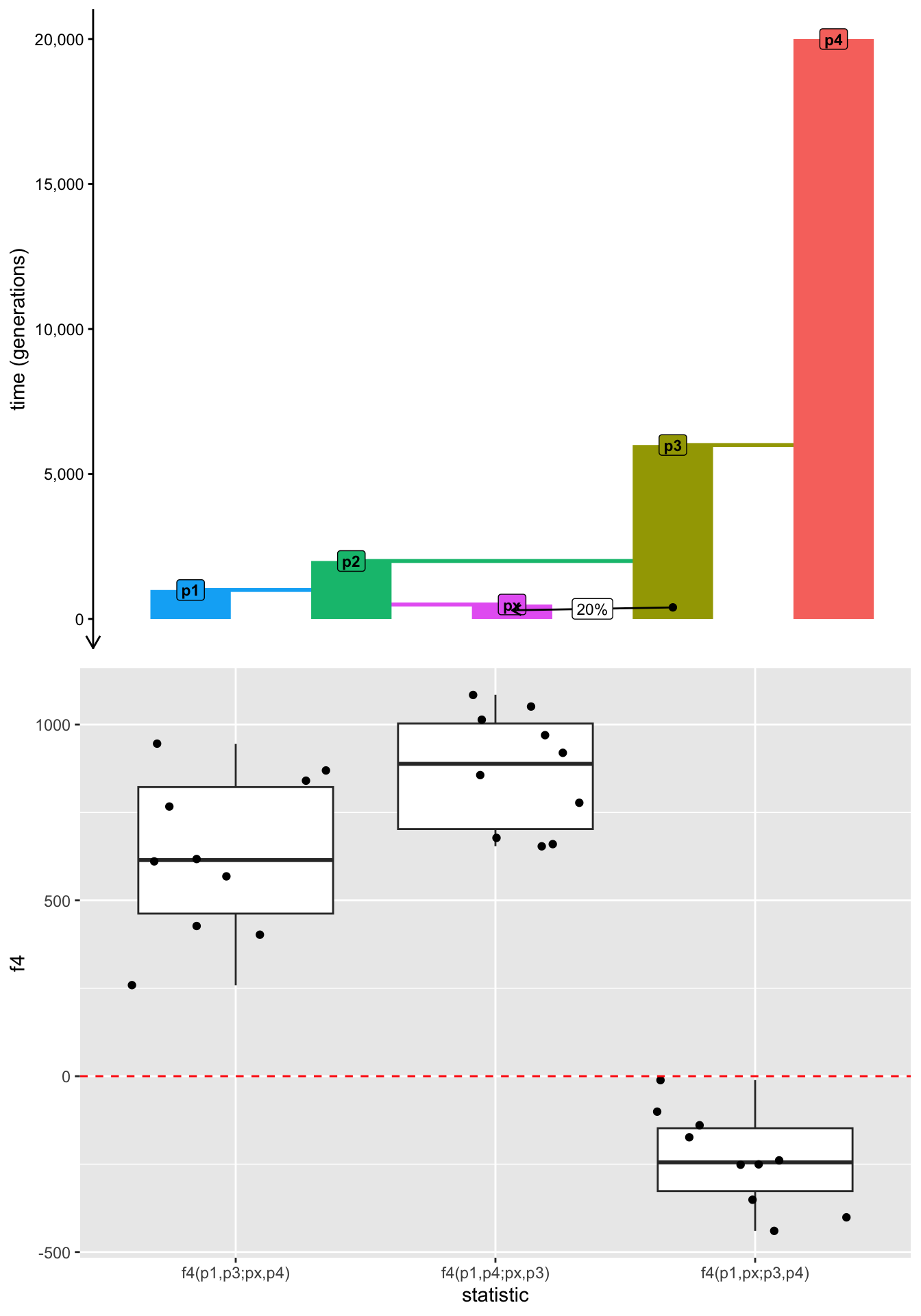
As we can see, because of the admixture event, our previously tree-like population model is no longer tree. In the tree model without an admixture edge, there was no path overlap between the pairs p1-px and p3-p4, which is why the \(f_4(p1,px;p3,p4)\) statistic was zero.
Admixture is a violation of “treeness”, because “mathematical” trees are not allowed to have edges (they effectively create “loops” in the trees)—structures which do have edges are instead called “admixture graphs”. This is why the statistic now significantly deviates from zero (and is negative).
This is exactly why \(f_4\) is useful as a statistical hypothesis test of admixture—if a population quartet is from a truly tree-like model, this statistic will always necessarily be zero; conversely, it can only ever be non-zero if the underlying model (usually hidden, in real-world applications) involves admixture which violates “treeness”.
Exercise: Estimating admixture proportions
From the little simulation and tree-doodling experiments, we now have a sense of how \(f\) statistics mathematically quantify allele frequency correlations between lineages of population trees and how they can be interpreted as the amounts of overlaps of paths traced along branches of those trees.
We also have an idea how different patterns emerge in \(f_4\) statistic expectations when gene-flow is introduced into population trees, adding admixture edges to them and turning them into so-called “admixture graphs”.
It turns out that the same principles allow us to not just test the hypothesis of whether an admixture event happened in the history of our samples, but also estimate the proportion of ancestry derived from this admixture—a concept known as \(f_4\)-ratio statistics.
The theory of \(f_4\)-ratios can get quite complex, but let’s try to get an idea about its internal workings using a very simple example and build up from there. We’ll end up inventing the \(f_4\)-ratio statistic from scratch!
Let’s consider our model again and set a goal to estimate how much ancestry of px came from p3 (or how much came from p2 into px—these are complementary, of course). Imagine tracing a path through the population from px to p2 through the tree. Draw a fresh sketch of our five-population model on paper, and trace this px-p2 path on it.
How many such paths can we take through the tree?
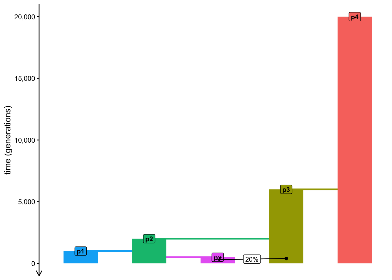
How many px to p2 paths would we have available if there wasn’t any admixture in the model?
Now that we’ve established that there are two possible paths from px to p2 in our admixture model, what is the interpretation of \(f_4(p1,p4;px,p2)\) at any given locus of the genome? What would be the possible values of this \(f_4\) in this situation? Again, try to use pen and paper to figure it out based on the knowledge of \(f_4\) as a measures of internal branches in a tree.
Hint: Remember that we’ve established that there are two possible paths from px to p2 in the tree, depending on whether px has a genetic ancestry coming from p2 or p3 at a given locus of the genome.
Now for the final punchline!
You’ve already established that one of the two interpretations of \(f_4(p1,p4;px,p2)\) describes the internal branch in the tree separating the pairs p1-p4 and px-p2, which exists for the parts of the genome which px inherited from p3 (the other interpretation giving a value of zero, by definition).
What is the interpretation of \(f_4(p1,p4;p3,p2)\)? Again, sketch the internal path represented by this \(f_4\) statistic in your tree model on paper.
Finally, what happens if you would take the value produced by \(f_4(p1,p4;px,p2)\) and divided it by \(f_4(p1,p4;p3,p2)\), i.e. what is the interpretation of the following equation?
\[\frac{f_4(p1,p4;px,p2)}{f_4(p1,p4;p3,p2)}\]
There’s one thing to be smart and logical, there’s one thing to be able to derive an equation (or be handed one equation from a paper or a textbook). Trusting and understanding the equation is another matter—that’s when simulations can be very useful again.
Use the equation for the \(f_4\)-ratio estimator of ancestry proportion to write a new code chunk in your f_admixture.R script which will simulate the values of this estimator expected from our admixture model using a ratio two individual ts_f4() statistics, specifying the quartet configuration accordingly. Then visualize the admixture proportion thus computed—did your estimator recover the known value of 20% of admixture?
If you want an extra challenge, it turns out there are multiple variations of how the ancestry proportion can be estimated. Try to find them, add them to your ts_replicate() code and compare them to one another by visualizing their distributions across all replicates.
NoteClick to see the solution
I managed to come up with three possible \(f_4\)-ratio variations, all three programmed and benchmarked below:
Variant number 1 is the one we derived together, based on tracing the path from
pxtop2through populationp3(this is predicted to estimate 20% ancestry).Variant number 2 is the complement to the first variant which traces the ancestry from
pxtop3through populationp2(and therefore is expected to estimate 80% ancestry).Variant number 3 is a little strange and I came up with it by accident when I was developing the very first \(f_4\) ratio exercise. Notice that although it does produce the correct 20% expectation, it shows a much higher variance (i.e., much more statistical noise).
props <- ts_replicate(
  n = 50,
  {
  ts <-
    msprime(model, sequence_length = 10e6, recombination_rate = 1e-8, schedule = schedule) %>%
    ts_mutate(mutation_rate = 1e-8)

  s <- ts_names(ts, split = TRUE)

  # variant #1 -- this is the variant we derived together
  num1 <- ts_f4(ts, W = s["p1"], X = s["p4"], Y = s["px"], Z = s["p2"])$f4
  den1 <- ts_f4(ts, W = s["p1"], X = s["p4"], Y = s["p3"], Z = s["p2"])$f4
  prop1 <- num1 / den1

  # variant #2
  num2 <- ts_f4(ts, W = s["p1"], X = s["p4"], Y = s["px"], Z = s["p3"])$f4
  den2 <- ts_f4(ts, W = s["p1"], X = s["p4"], Y = s["p2"], Z = s["p3"])$f4
  prop2 <- num2 / den2

  # variant #3 (a weird one?)
  num3 <- ts_f4(ts, W = s["p1"], X = s["px"], Y = s["p2"], Z = s["p4"])$f4
  den3 <- ts_f4(ts, W = s["p1"], X = s["p3"], Y = s["p2"], Z = s["p4"])$f4
  prop3 <- - num3 / den3

  # create a data frame with different variants
  data.frame(
    proportion = c("variant1", "variant2", "variant3 (weird one?)"),
    value = c(prop1, prop2, prop3)
  )
  }
)

p_model <- plot_model(model, proportions = TRUE)

p_f4ratios <- ggplot(props, aes(value, color = proportion)) +
    geom_density() +
    geom_vline(xintercept = c(0.2, 0.8), linetype = "dashed", color = "red") +
    coord_cartesian(xlim = c(0, 1)) +
    labs(title = "Simulation-based validation of f4-ratio ancestry estimates",
         subtitle = "(three different variations of f4-ratios are shown)",
         x = "ancestry proportion") +
    theme(legend.position = "bottom")

p_ratios <- plot_grid(p_model, p_f4ratios, nrow = 2)

p_ratios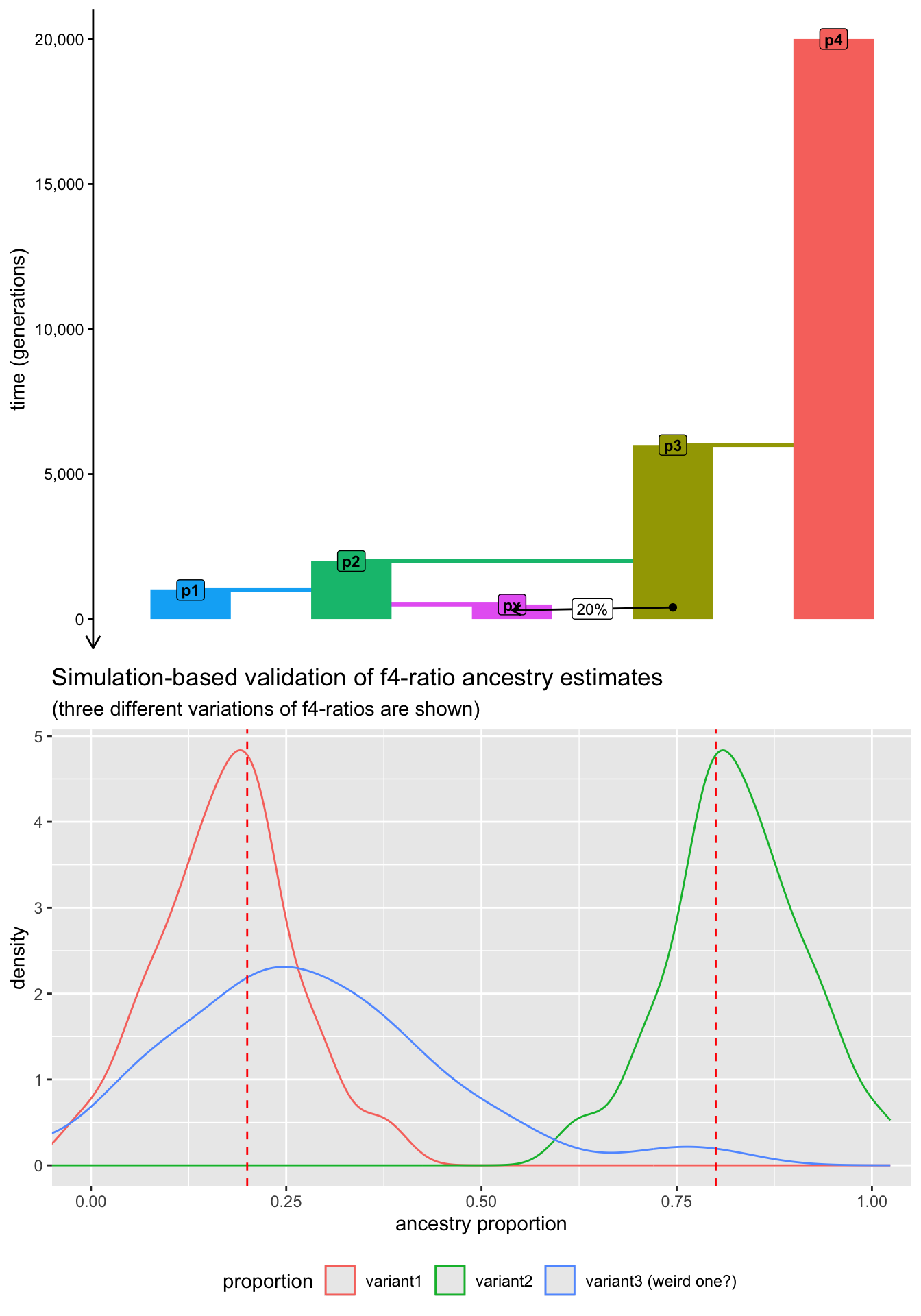
Note that there’s still a lot of variance and noise. In a practical setting, we would run many more simulation replicates (100 or even more) for genomes much longer than just 10 Mb (for instance, even 100 Mb). We don’t do this here because those simulations would take too long to do on a normal laptop.
Catching up
This was even more work! And no wonder—a simulation-based analysis like this one could easily be part of a real research paper. In fact, many studies which introduced these theoretical concepts used these simulations as proof-of-principle, and increasing number of applications include them for benchmarking and validation of results. Now you know how to do these things as well!
If you want to see the state of the final f_admixture.R script, you can find it below.
Exercise: What are tree sequences?
We’ve mentioned the concept of a “tree sequence” many times but until this chapter, we haven’t considered tree-thinking very explicitly. Indeed, for most of our daily practical work, we don’t need to be aware of the underlying tree-sequence data that much, but it’s always a good idea to know what’s going on behind the scenes of the methods that we use. Let’s take a small peek at what actually is hiding behind our familiar ts objects in practice. This section will be more like a demonstration rather than a “serious exercise”, just in case you’re curious about this topic.
When you type ts into your R console, you’ll get a summary of the most important characteristics in your data. For instance, consider a small 1 Mb tree-sequence simulation like this, and note the number of trees, the number of edges, nodes, and mutations:
schedule <- schedule_recording(model, times = 0, list("each", 1))

ts <-
    msprime(model, sequence_length = 1e6, recombination_rate = 1e-8, schedule = schedule, random_seed = 42) %>%
    ts_mutate(mutation_rate = 1e-8, random_seed = 42)

ts
╔═══════════════════════════╗
║TreeSequence ║
╠═══════════════╤═══════════╣
║Trees │ 247║
╟───────────────┼───────────╢
║Sequence Length│ 1,000,000║
╟───────────────┼───────────╢
║Time Units │generations║
╟───────────────┼───────────╢
║Sample Nodes │ 10║
╟───────────────┼───────────╢
║Total Size │ 64.2 KiB║
╚═══════════════╧═══════════╝
╔═══════════╤════╤═════════╤════════════╗
║Table │Rows│Size │Has Metadata║
╠═══════════╪════╪═════════╪════════════╣
║Edges │ 838│ 26.2 KiB│ No║
╟───────────┼────┼─────────┼────────────╢
║Individuals│ 5│164 Bytes│ No║
╟───────────┼────┼─────────┼────────────╢
║Migrations │ 0│ 8 Bytes│ No║
╟───────────┼────┼─────────┼────────────╢
║Mutations │ 332│ 12.0 KiB│ No║
╟───────────┼────┼─────────┼────────────╢
║Nodes │ 220│ 6.0 KiB│ No║
╟───────────┼────┼─────────┼────────────╢
║Populations│ 5│373 Bytes│ Yes║
╟───────────┼────┼─────────┼────────────╢
║Provenances│ 2│ 4.3 KiB│ No║
╟───────────┼────┼─────────┼────────────╢
║Sites │ 332│ 8.1 KiB│ No║
╚═══════════╧════╧═════════╧════════════╝We can extract a single tree at a given index using the function ts_tree(). (Note that because slendr ties into the Python module tskit behind the scenes, indexing into the tree sequence starts at 0.) This doesn’t give us much information though—it’s just an opaque object in computer memory, but we don’t see anything interesting when we type the tree variable into the R console:
tree <- ts_tree(ts, i = 0)
tree
<tskit.trees.Tree object at 0x11584ae70>We can use the built-in slendr helper function ts_draw() to visualize these tree objects. For instance, here’s how we can visualize the 0th (i.e., the first) tree in our small tree sequence. Note that by setting labels = TRUE, we can see individuals’ names at the leaves of the tree, as well as the fact that each individual is represented by two leaves (one for each of its two chromosomes).
ts_draw(tree, labels = TRUE, width = 1000, height = 500, title = paste("Tree #", tree$index))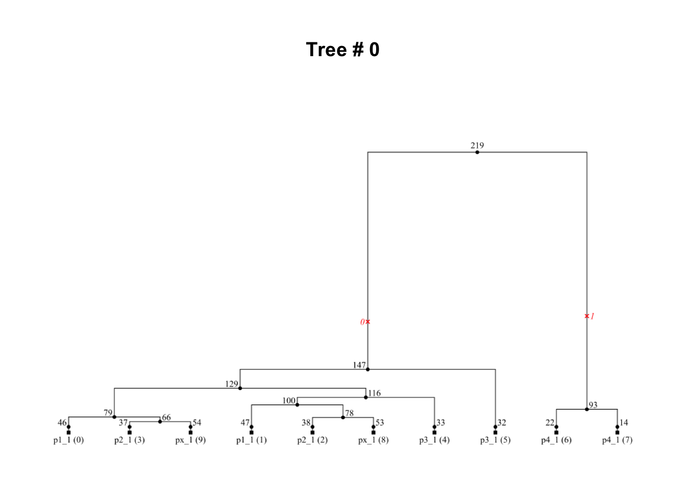
Take a few minutes visualizing different trees, perhaps starting from 0th and going forward, until you get bored!
As you do this, notice that “neighboring” trees tend to be quite similar (why do you think this is?).
Can you find an example of a tree which fits our underlying population tree model?
How about trees which clearly “contradict” this model? Can you find any?
How about a tree which would show evidence of gene flow from
p3topxwe programmed in our model? Can you find one?You might encounter red cross signs plotted on the trees—what do they represent?
The outcome of an evolutionary simulation is completely random, so don’t get too frustrated if you don’t find lots of meaningful information while doing this. At the very least, when you explore the trees along the tree sequence, even for a small section of a genome like 1 Mb in this case, it makes you appreciate just how complex real-world evolutionary processes are.
If you want to explore the exact same tree-sequence that I had, you can download it with the following commands and use it instead of your simulated ts object:
NoteClick to see the solution
Here’s what I found after a couple of minutes of visualizing different trees in my tree sequence:
- A neat and tidy genealogy which is completely concordant with our population tree (take a look at the tip labels with population names and compare this tree to the overall population tree model we worked with in this chapter):
i <- 203
tree <- ts_tree(ts, i)
ts_draw(tree, labels = TRUE, width = 1000, height = 500, title = paste("Tree #", tree$index))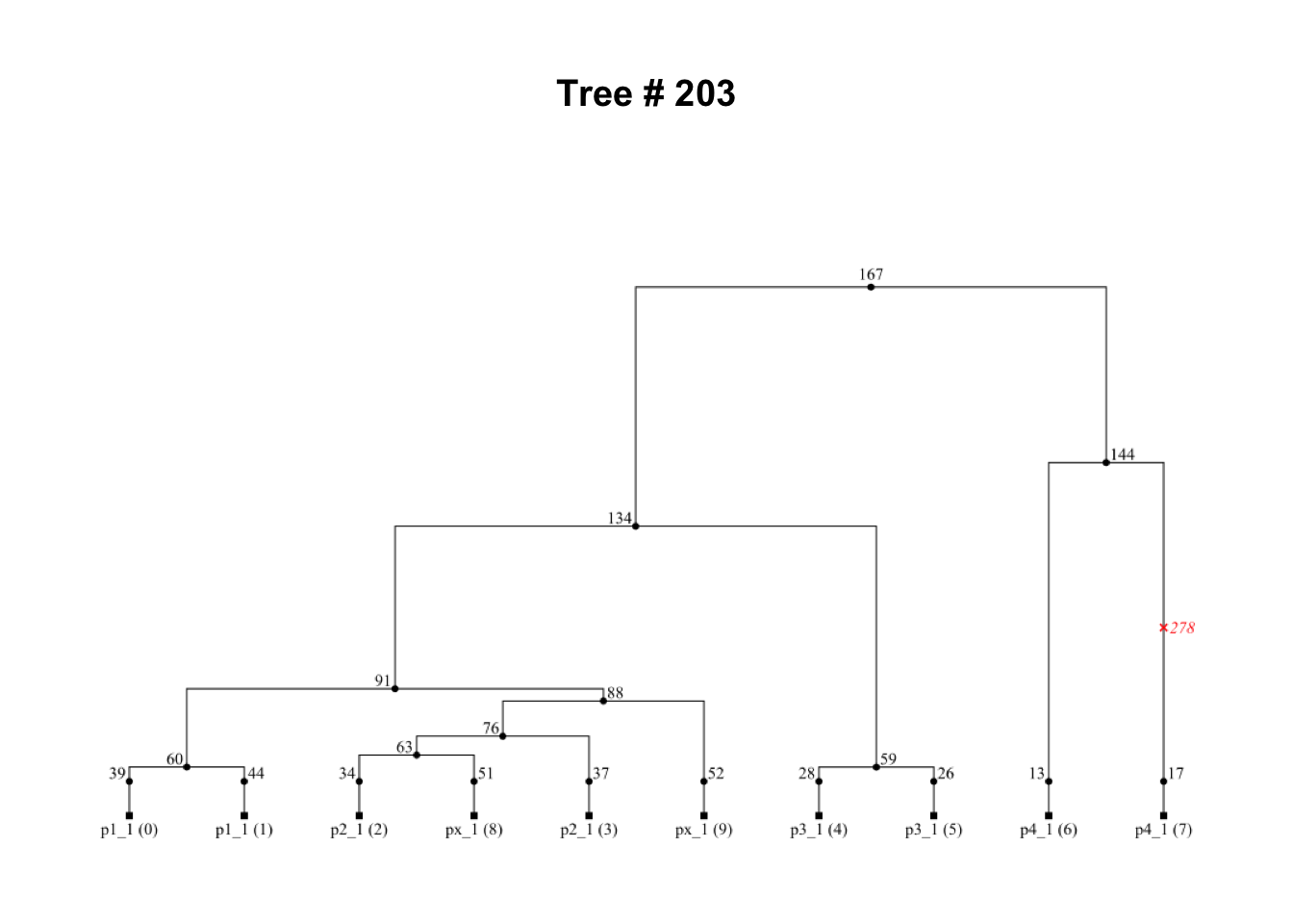
We can also see that the tree immediately after this one is basically the same. This is because of a single (ancient) recombination event which only affected one branch in the tree, but the remainder of the genealogy stays the same (because recombination didn’t affect those individuals’ ancestors):
i <- 204
tree <- ts_tree(ts, i)
ts_draw(tree, labels = TRUE, width = 1000, height = 500, title = paste("Tree #", tree$index))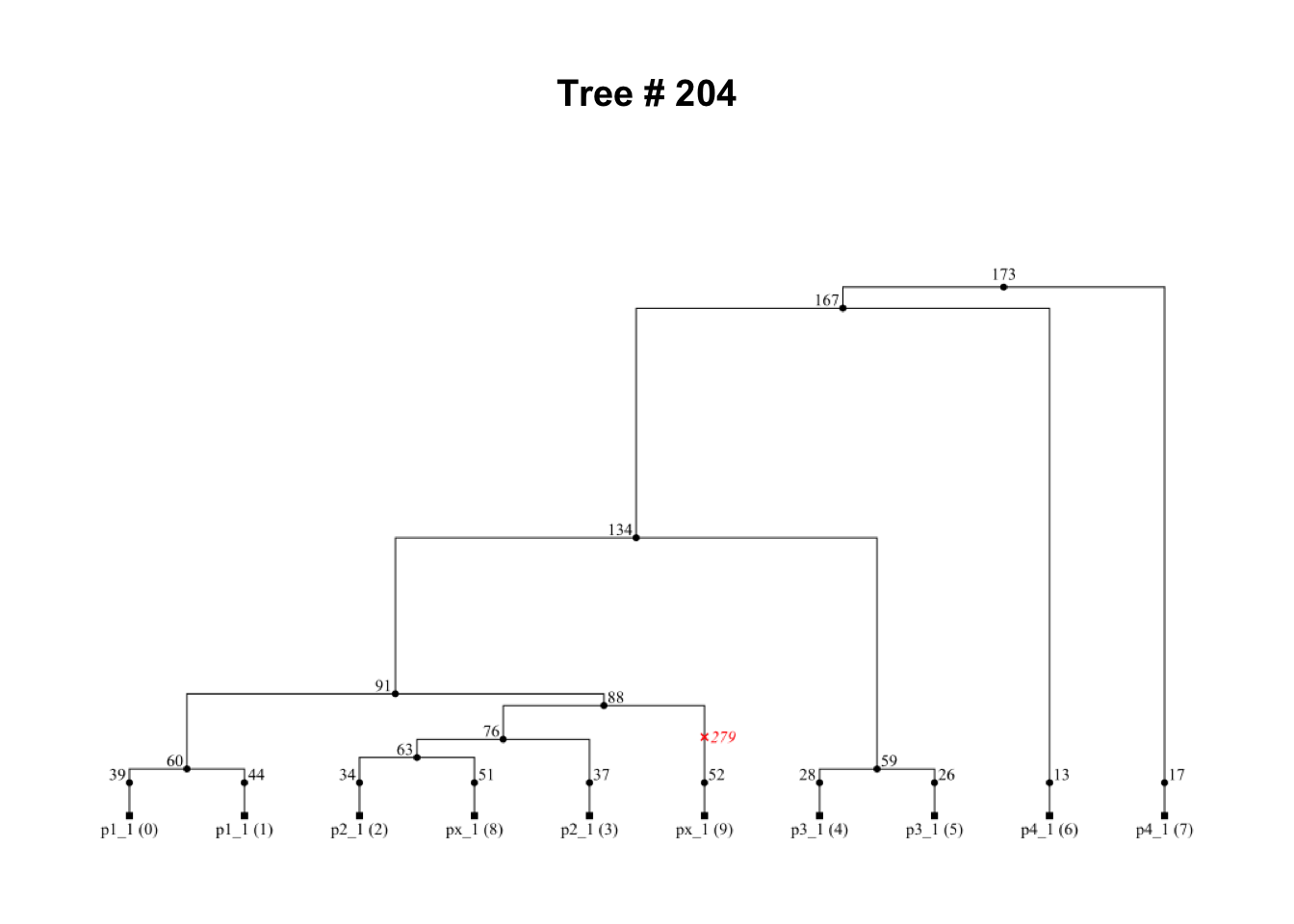
- A tree showing a clear evidence of gene flow from
p3intopx:
i <- 243
tree <- ts_tree(ts, i)
ts_draw(tree, labels = TRUE, width = 1000, height = 500, title = paste("Tree #", tree$index))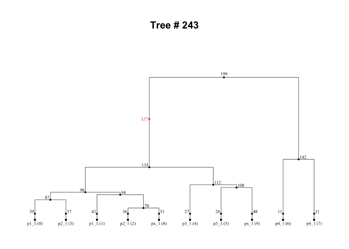
- Another locus in the genome carries a tree which is an utter mess and doesn’t seem to be similar to our underlying population tree model at all:
i <- 114
tree <- ts_tree(ts, i)
ts_draw(tree, labels = TRUE, width = 1000, height = 500, title = paste("Tree #", tree$index))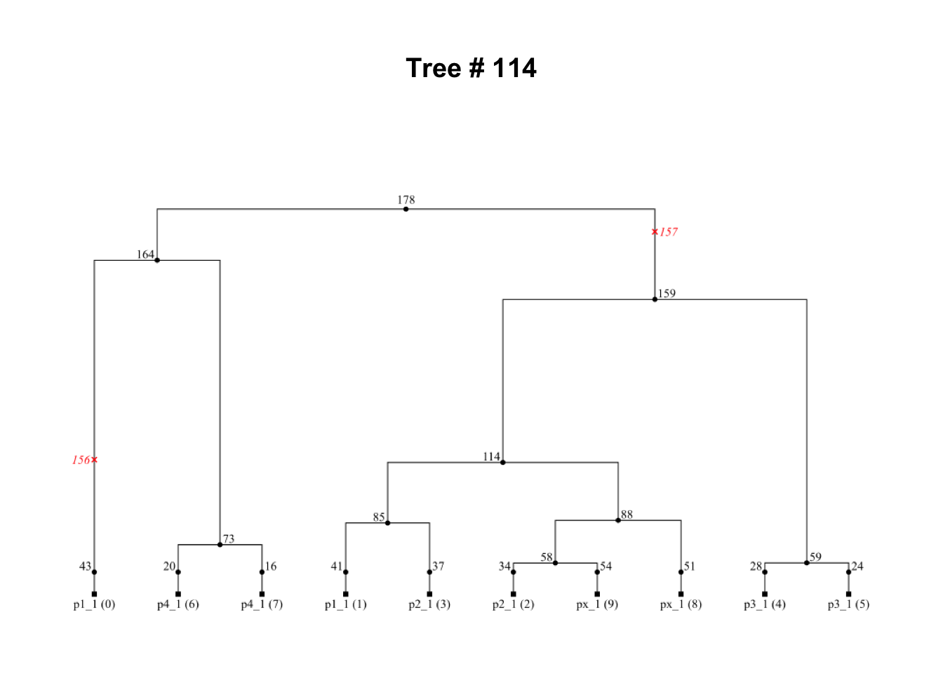
Oh, and the red crosses represent mutations!
I hope that this little exercise illustrates nicely just how much work population genetic statistics do for us in understanding the hidden truth behind real-world evolutionary processes—they do this by aggregating massive amounts of convoluted genealogical data resulting from these processes, and help us extract and see meaningful patterns in them.
Bonus exercise (if you want a programming challenge)
When playing with \(f\)-statistics in this chapter, you’ve probably noticed various symmetries in \(f_4\) (but also other \(f\)-statistics) depending on the arrangement of their “configuration” (order of populations). As a trivial example, an \(f_3(A; B, C)\) and \(f_3(A; C, B)\) will give you exactly the same value.
Try to figure out how many unique \(f_4\) values involving a single quartet (for instance, quartets involving different permutations of p1, p2, p3, and p4 populations) are there. How about how many absolute values? You could answer this by drawing and doodling on paper, but try to use computer simulations to do this too! You can program whatever demographic model you’d like for this purpose—the specifics don’t matter much as long as the model has some four populations involved.