library(slendr)
init_env()

outgroup <- population("outgroup",   time = 7000000, N = 10000)

ancestor <- population("ancestor",   time = 6000001, N =  1000, parent = outgroup, remove = 599999)

altai    <- population("Altai",      time =  600000, N =  1000, parent = ancestor, remove = 49999)
vindija  <- population("Vindija",    time =  200000, N =  1000, parent = altai, remove = 49999)

san      <- population("San",        time =  600000, N = 10000, parent = ancestor)
mbuti    <- population("Mbuti",      time =  350000, N = 10000, parent = san)
yoruba   <- population("Yoruba",     time =  220000, N = 10000, parent = mbuti)
dinka    <- population("Dinka",      time =  150000, N = 15000, parent = yoruba)

nonafr   <- population("nonAfrican", time =   70000, N = 3000,  parent = dinka)

gf <- gene_flow(from = vindija, to = nonafr, proportion = 0.03, start = 55000, end = 50000)

model <- compile_model(
  populations = list(outgroup, ancestor, altai, vindija, san, mbuti, yoruba, dinka, nonafr),
  gene_flow = gf,
  generation_time = 30
)

# schedule recording of present-day individuals
schedule_present <- schedule_recording(
  model, times = 0,
  list(outgroup, 1), list(san, 1), list(mbuti, 1), list(yoruba, 1), list(dinka, 1), list(nonafr, 1)
)

# schedule recording of two Nenderthals
schedule_neand <- schedule_recording(model, times = 50000, list(altai, 1, "Altai"), list(vindija, 1, "Vindija"))

# schedule recording of Upper-Paleolithic modern humans
schedule_emh <- schedule_recording(model, times = runif(n = 50, min = 1000, max = 45000), list(nonafr, 1))

# bind the schedules into one
schedule <- rbind(schedule_present, schedule_neand, schedule_emh)

ts <-
  msprime(model, sequence_length = 100e6, recombination_rate = 1e-8, schedule = schedule) %>%
  ts_mutate(mutation_rate = 1e-8)

s <- ts_names(ts, split = TRUE)Neanderthal ancestry trajectory
In this case study, you will be reproducing an important result from my 2018 study on the limits of selection against Neanderthal introgression. In a very unplanned and unpredictable manner, this research ended up turning into a study on the importance of model assumptions on the robustness of inferences with \(f_4\) statistics and how they can produce entirely misleading inferences about ancient admixture events in human history.
I chose this case study for several reasons:
This research would’ve been absolutely impossible without simulations exactly like those you’ve learned to do in this workshop.
The limitations of computational tools I had available at the time required me to write hundreds of lines of code spread across shell scripts, Python scripts, and R scripts. Thanks to slendr, a project which required months of work and lots of coding is possible to do in a handful of lines of R.
It provides an excellent educational example of how slendr simulations can help you navigate practically any demographic scenario, gain confidence in your results, and aid in their interpretation.
Most importantly, the lessons of my paper apply in any context of using \(f_4\) statistics in ancient DNA research. The Neanderthal introgression case serves just as an illustrative example.
Preparation
To avoid too much frustration with transcribing very complex admixture graph model from yet another of my drawings, please copy the following code into a new script introgression.R. When you visualize the model, you should see a relatively detailed (yet still simplified) model of ancient human history including Neanderthal introgression into the ancestors of non-Africans. Again, please inspect this script to make sure you understand what it does—this is now even more important than before.
Please note that real-world simulations are rather computationally intensive, much more so than the modeling we did in our exercises. Generally speaking, most of simulation-based research happens on big computational servers. For our learning purposes here, if things take too long, just lower the amount of simulated sequence. However, be aware that this will, in turn, make statistics much more noisy (but that’s OK, we’re learning here).
NoteClick to see the the script
introgression.R
In case your simulation takes too long or your computer seems to be struggling, you can replace your tree-sequence simulation command by this bit of code which reads my simulated ts object from the internet. Then, continue working with it as if you had simulated it yourself.
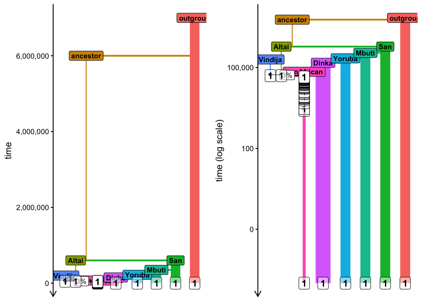
Here’s the model visualization (very janky, I know, but it is what it is…):
cowplot::plot_grid(
  plot_model(model, proportions = TRUE, schedule = schedule),
  plot_model(model, proportions = TRUE, schedule = schedule, log = TRUE),
  ncol = 2
)
And here are the individuals we “sequenced”, as a sanity check (mostly because of how hard-to-read the model visualization above is):
ts_recorded(ts) %>% print(n = Inf)# A tibble: 58 × 3
name time pop
<chr> <dbl> <chr>
1 Altai 50000 Altai
2 Vindija 50000 Vindija
3 nonAfrican_1 44817 nonAfrican
4 nonAfrican_2 44547 nonAfrican
5 nonAfrican_3 43198 nonAfrican
6 nonAfrican_4 42490 nonAfrican
7 nonAfrican_5 41708 nonAfrican
8 nonAfrican_6 41350 nonAfrican
9 nonAfrican_7 39128 nonAfrican
10 nonAfrican_8 38995 nonAfrican
11 nonAfrican_9 38420 nonAfrican
12 nonAfrican_10 37994 nonAfrican
13 nonAfrican_11 36537 nonAfrican
14 nonAfrican_12 35012 nonAfrican
15 nonAfrican_13 31968 nonAfrican
16 nonAfrican_14 30783 nonAfrican
17 nonAfrican_15 30133 nonAfrican
18 nonAfrican_16 29967 nonAfrican
19 nonAfrican_17 28768 nonAfrican
20 nonAfrican_18 28251 nonAfrican
21 nonAfrican_19 26562 nonAfrican
22 nonAfrican_20 26423 nonAfrican
23 nonAfrican_21 24809 nonAfrican
24 nonAfrican_22 23667 nonAfrican
25 nonAfrican_23 22767 nonAfrican
26 nonAfrican_24 22107 nonAfrican
27 nonAfrican_25 21172 nonAfrican
28 nonAfrican_26 20199 nonAfrican
29 nonAfrican_27 19127 nonAfrican
30 nonAfrican_28 18576 nonAfrican
31 nonAfrican_29 17861 nonAfrican
32 nonAfrican_30 16905 nonAfrican
33 nonAfrican_31 15371 nonAfrican
34 nonAfrican_32 15069 nonAfrican
35 nonAfrican_33 13050 nonAfrican
36 nonAfrican_34 12749 nonAfrican
37 nonAfrican_35 12265 nonAfrican
38 nonAfrican_36 9932 nonAfrican
39 nonAfrican_37 9758 nonAfrican
40 nonAfrican_38 9626 nonAfrican
41 nonAfrican_39 9570 nonAfrican
42 nonAfrican_40 6174 nonAfrican
43 nonAfrican_41 5658 nonAfrican
44 nonAfrican_42 5500 nonAfrican
45 nonAfrican_43 5489 nonAfrican
46 nonAfrican_44 5015 nonAfrican
47 nonAfrican_45 4161 nonAfrican
48 nonAfrican_46 4033 nonAfrican
49 nonAfrican_47 3584 nonAfrican
50 nonAfrican_48 2116 nonAfrican
51 nonAfrican_49 1178 nonAfrican
52 nonAfrican_50 1114 nonAfrican
53 Dinka_1 0 Dinka
54 Mbuti_1 0 Mbuti
55 San_1 0 San
56 Yoruba_1 0 Yoruba
57 nonAfrican_51 0 nonAfrican
58 outgroup_1 0 outgroup Indirect \(f_4\)-ratio estimate of Neanderthal ancestry
The main controversy at the time I did this research was caused by the observation that ancient DNA time series of early modern humans (like the one you just simulated!) showed a clear decline in Neanderthal ancestry trajectory over the past ~45 thousand years.
The way the authors of the “Neanderthal decline” paper computed Neanderthal ancestry was using what I ended up naming as the “indirect \(f_4\)-ratio” estimate, described in panel B of Figure 1 in my paper (where “Dinka” typically represented the “East African” lineage, and “Yoruba” represented the “Central and West African” lineage, to follow the terminology in that schematic diagram). This “indirect” estimate is what showed clear evidence of the decline in Neanderthal ancestry over time.
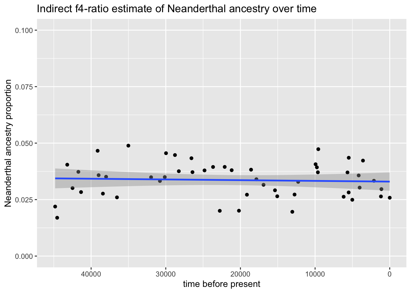
Compute this “indirect \(f_4\)-ratio” estimate of Neanderthal ancestry from your simulated ts tree sequence for every one of your “nonAfrican” individuals. Then visualize the simulated Neanderthal ancestry trajectory as a time-series (i.e., your indirect ancestry estimate on the y-axis, time on the x-axis), similarly to what’s shown for the empirical data linked above. What kind of temporal trend do you observe?
Hint: You can either compute this “manually” using the path overlap principles described in the \(f\) statistics chapter earlier, or you can make your life a bit easier and use a dedicated slendr function ts_f4ratio(). That function follows the same nomenclature shown in my Figure 1B diagram above. If you use ts_f4ratio(), be aware that X can only always be one individual in this function, so you will want to compute this for every aDNA individual in the time-series separately.
Hint: If you need more help, see this example of how to compute the indirect \(f_4\)-ratio for a single individual.
NoteClick to see the solution
Here’s what my simulated trajectory looks like:
Adding complex admixture during modern human prehistory
In your visualization of the indirect \(f_4\)-ratio trajectory, you should have noticed no trend at all. Indeed, under neutrality, Neanderthal ancestry is expected to constant throughout the millenia. However, the puzzle at the time was that the empirical data showed clear, significant temporal decline in this estimate over time!
The solution to the puzzle came out of (lots of) simulations and modeling, very similar to what you’ve done in this workshop so far. Let’s retrace my steps again.
What happens if you introduce additional gene flow events within the modern human population tree? For example, simulate admixture between the two African lineages used in your indirect \(f_4\)-ratio calculation, as well as “back-flow” admixture from the non-African population into both of those African lineages. Let’s say that all of these admixture events should happen at 5% proportion, the within-Africa gene flow should happen starting from 20 kya until present-day time 0, and the backflow nonAfrican admixture should happen from 8 kya to 5 kya.
None of those changes into the demographic model changes the amount of true Neanderthal ancestry in Europeans. But what does the trajectory of the indirect Neanderthal ancestry estimate look like when you compute it on this model with additional complex admixture within modern humans?
Hint: Feel free to make a copy of your introgression.R script to make the indicated changes, perhaps saving it as introgression_complex.R, just to make things clean and tidy.
Again, if you think your tree-sequence simulation takes too long or that your computer is struggling, feel free to use this chunk of code to read my own ts tree sequence from the internet, then continue working with it as if you simulated it yourself:
NoteClick to see the solution
Here’s what my simulated trajectory looks like on the modified model:
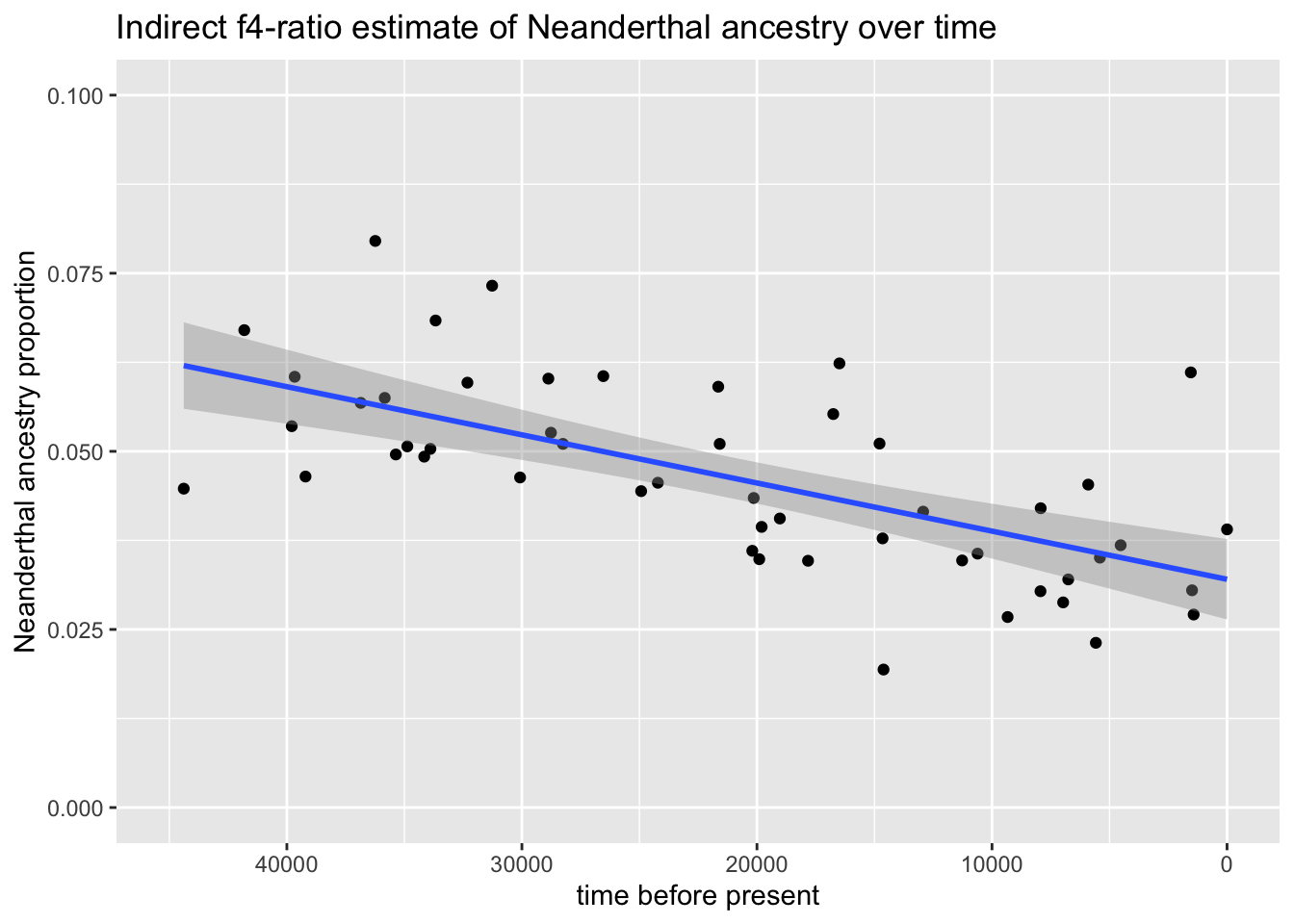
We pick up a decline in Neanderthal ancestry even though we know there’s no decline at all! This is because the indirect \(f_4\)-ratio make very strong assumptions about the population tree of modern humans, specifically the fact that there was no admixture between different modern human lineages after Neanderthal introgression.
Don’t worry if your own result is noisy! That’s what replicate simulations are for (remember the existence of the ts_replicate() function, which I wrote exactly for this purpose).
Direct \(f_4\)-ratio estimate of Neanderthal ancestry
The reason we had to compute Neanderthal ancestry using the “indirect” statistic is because we only had a single Neanderthal genome available at the time—the genome of the “Altai” Neanderthal.
Luckily, a few years later, a second Neanderthal was sequenced which allowed us to express the \(f_4\)-ratio estimate in a “direct” way using both Neanderthal genomes. We called this estimate the “direct \(f_4\)-ratio” estimate.
If you got to the relevant part of the \(f\)-statistics chapter, you may remember that we discovered multiple ways of computing the px ancestry—either coming from the p3 population (we could call it alpha), or as its complement coming from the p2 population (we could compute it as 1 - alpha). Well, the “indirect vs direct \(f_4\)-ratio” situation is exactly the same.
Using this idea, compute the “direct \(f_4\)-ratio” using the two Neanderthal genomes on the model which includes lots of complex admixture within modern humans. How does the direct \(f_4\)-ratio perform on such a model? Is it robust and can it infer the Neanderthal ancestry trajectory accurately, unlike the indirect estimate?
Hint: If you need help, see this example of how to compute the direct \(f_4\)-ratio for a single individual again.
NoteClick to see the solution
Here’s what my simulated trajectory looks like on the modified model:
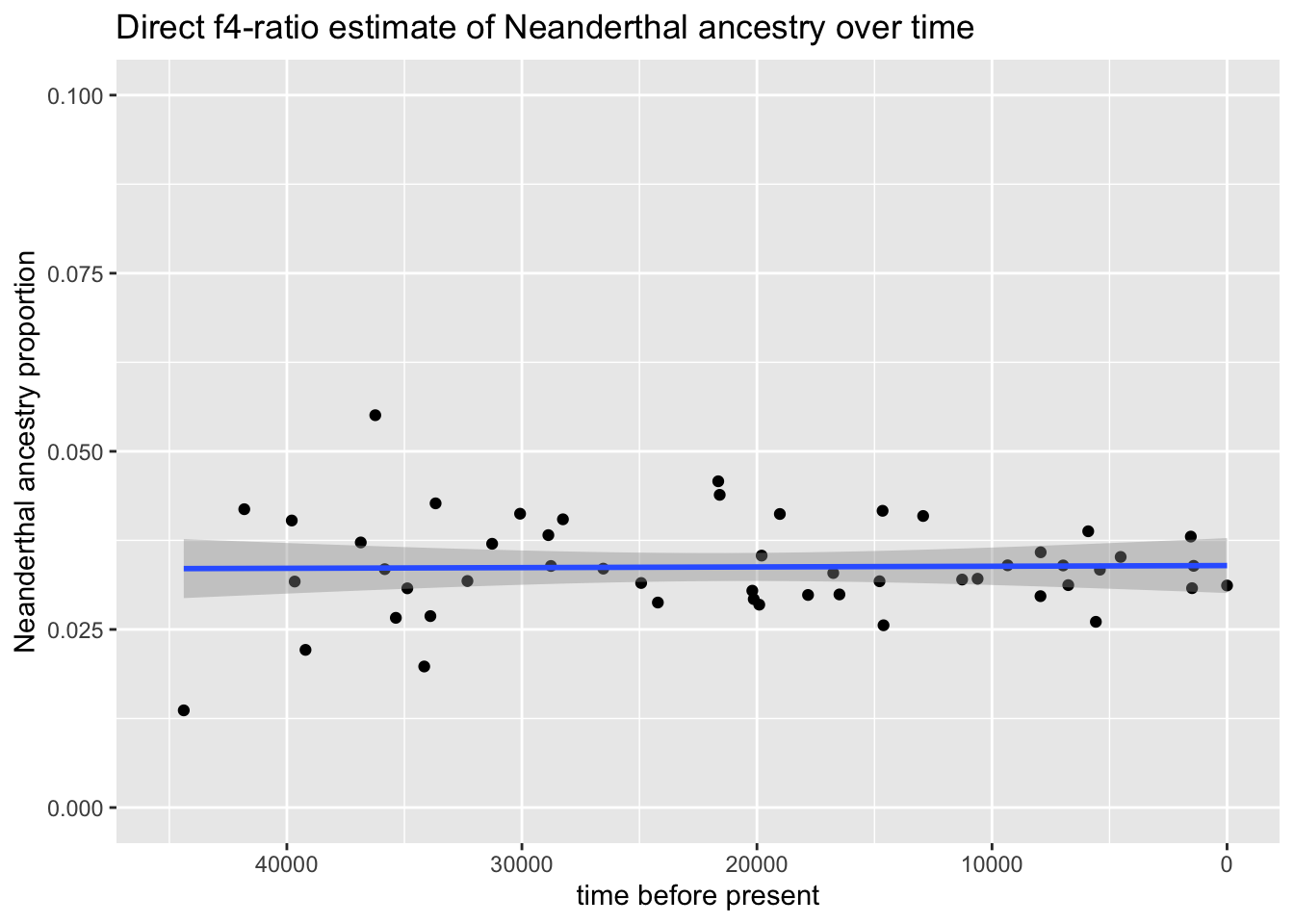
Don’t worry if your own result is noisy! That’s what replicate simulations are for (remember the existence of the ts_replicate() function, which I wrote exactly for this purpose).
Finally, here’s a comparison of both indirect and direct \(f_4\)-ratio statistics against one another. Again, bear in mind that in reality (which we know from the simulations) the proportion of Neanderthal ancestry remained the same over tens of thousands of years—but the indirect \(f_4\)-ratio statistic gives us a misleading result, because it makes assumptions about modern human population relationships which simply do not hold:
`geom_smooth()` using formula = 'y ~ x'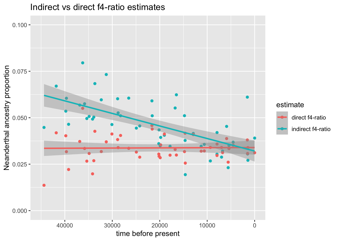
In conclusion, the demographic simulation exploration in my paper took months of work (and a combination of Python simulations, shells scripts, and R data analysis scripts), resolving a problem which occupied the brightest minds of population genetics at the time. I hope that the fact that you’re able to reproduce the core aspects of this work this easily convinces you of the power of slendr modeling for this type of research!
Bonus exercise
Because I saved you a lot of work by providing the introgression admixture model already programmed, here’s a bonus challenge:
One question that the authors of the original draft Neanderthal genome paper had to answer was the issue of the direction of gene-flow.
How would you show that introgression happened from Neanderthals into non-Africans and not the other way around? Skim through the paper linked above, particularly focusing on the section called “Direction of gene flow” to get an idea of how did the authors distinguished the two scenarios using a \(D\) statistic (which, for our purposes, could be thought of as essentially equivalent to the \(f_4\) statistic as we’ve established it, so you can use the familiar \(f_4\) to answer this question).
Hint: They used logic to argue for what would the expected values of certain \(f_4\) statistics look like between two different models (the model of introgression from Neanderthals into non-Africans, and the model of introgression from non-Africans into Neanderthals). We want to use simulations to try to arrive at the same conclusions.