library(slendr)
init_env()

pop <- population("pop", time = 2001, N = 5000)

model <- compile_model(populations = pop, generation_time = 1, direction = "backward")

plot_model(model)

ts <- msprime(model, sequence_length = 10e6, recombination_rate = 1e-8)

samples <- ts_names(ts)Within-population statistics
Theme of this chapter
Now that we have a slendr model encoded in a reproducible R script and a simulated genomic data in the form of a tree sequence ts, how can we compute population genetic statistics from this data?
Computing statistics requires a specification of what should be computed and how. For instance, which individuals should a computation be performed on? If groups of multiple individuals are involved then how do we group them?
Exercises in this chapter will demonstrate these techniques using the most fundamental concepts of population genomics, namely \(N_e\), nucleotide diversity, and allele frequency spectrum. Rather than delving into the mathematical underpinning of these statistics, they will be used to provide a familiar context to show how easy it is to gain insight into (sometimes unintuitive) behavior of statistics in general through simulation-based exploration.
More concretely, the coding exercises will focus on the testing of a hypothetical inference method (using a toy example of \(N_e\) inference) using simulation-based benchmarking across a parameter grid.
Literature
In case you find yourself with extra time for some background reading, I recommend the following two chapters from the absolutely brilliant, freely-available textbook called “An Owner’s Guide to the Human Genome”. I don’t think there’s better companion resource on population genomics theory to what I’m trying to do in this practical, simulation-based workbook.
Chapter 2.1, “Genetic Drift: What happens to alleles over time?”: A beautiful and simple introduction to the concept of effective population size, the effect of genetic drift and mutation on the amount genetic diversity in a population, Wright-Fisher model, etc. (i.e, the core ideas we explore in this chapter through population genomic simulations).
Chapter 2.2, “More on genetic drift: The coalescent.”: A slightly more technical (yet still very easy to digest) dive into the coalescent theory background of the topics introduced in the previous chapter (and, therefore, also to the simulation exercises in this chapter), including discussion of the allele frequency spectrum (AFS).
Preparation
Let’s start with the following single-population model to be able to exclusively focus on statistics without having to deal with complexities of demographic modeling itself.
Restart your R session (Session -> Restart R), then look through the code below to understand what it does and save it as slendr_statistics.R. Run the entire script and inspect the produced visualization to make sure your understanding of this toy model was correct.
Exercise 1: Adding mutations
When you typed ts in your R console earlier, you may have noticed a strange thing — although msprime() simulated genomic data, there are no mutations! How can this be? Just take a look the tree-sequence summary below (specifically, the “Mutations” field):
ts╔═══════════════════════════╗
║TreeSequence ║
╠═══════════════╤═══════════╣
║Trees │ 17,787║
╟───────────────┼───────────╢
║Sequence Length│ 10,000,000║
╟───────────────┼───────────╢
║Time Units │generations║
╟───────────────┼───────────╢
║Sample Nodes │ 10,000║
╟───────────────┼───────────╢
║Total Size │ 4.4 MiB║
╚═══════════════╧═══════════╝
╔═══════════╤══════╤═════════╤════════════╗
║Table │Rows │Size │Has Metadata║
╠═══════════╪══════╪═════════╪════════════╣
║Edges │87,162│ 2.7 MiB│ No║
╟───────────┼──────┼─────────┼────────────╢
║Individuals│ 5,000│136.7 KiB│ No║
╟───────────┼──────┼─────────┼────────────╢
║Migrations │ 0│ 8 Bytes│ No║
╟───────────┼──────┼─────────┼────────────╢
║Mutations │ 0│ 16 Bytes│ No║
╟───────────┼──────┼─────────┼────────────╢
║Nodes │32,567│890.5 KiB│ No║
╟───────────┼──────┼─────────┼────────────╢
║Populations│ 1│222 Bytes│ Yes║
╟───────────┼──────┼─────────┼────────────╢
║Provenances│ 1│ 1.5 KiB│ No║
╟───────────┼──────┼─────────┼────────────╢
║Sites │ 0│ 16 Bytes│ No║
╚═══════════╧══════╧═════════╧════════════╝As we will see later, the magic of tree sequences allows us to compute any population genetic statistic without mutations. That said, for comparing simulated results to statistics computed by various third-party software outside of R, having mutations is often useful. Here’s how we can make that happen.
Modify the msprime(...) command in your script slendr_statistics.R by “piping” its output to ts_mutate(mutation_rate = 1e-8) (remember the %>% “pipe operator” introduced earlier). After you execute this new command and type ts in the R console to inspect the summary, you should see that mutations have been added. Verify that this is the case by typing ts in your R console.
Even though mutations are generally not needed, there’s almost never any huge downside to adding them, so I recommend you always use both msprime() and ts_mutate() in your models in this workshop.
With that out of the way, let’s proceed with computing population genetic statistics using slendr and tskit.
Exercise 2: Within-group(s) statistics — nucleotide diversity
The simplest possible computation we can do is to compute a statistic for a single population. As an example, let’s look at nucleotide diversity (also known as \(\pi\)), implemented by the slendr function ts_diversity().
If you look at its help page under ?ts_diversity, you will see that it accepts several arguments—for now let’s focus on the first two, ts = (which is obviously a tree-sequence object, such as the one produced by the msprime() engine) and sample_sets =.
Compute ts_diversity() on a single simulated individual, such as the individual with the name “pop_1”, by providing this name as the sample_sets = argument of this function. Knowing that slendr simulates diploids and knowing the definition of nucleotide diversity, how would you interpret the result that you get for this one individual from the perspective of genomics?
Now run the following three commands, one after the other. They look extremely similar, right? Do they produce the same value? If not, based on the results you get from each of those commands, can you deduce a general rule for how slendr interprets what it gets in the sample_sets = argument?
ts_diversity(ts, sample_sets = c("pop_1", "pop_42"))
ts_diversity(ts, sample_sets = list(c("pop_1", "pop_42")))
ts_diversity(ts, sample_sets = list(pop_subset = c("pop_1", "pop_42")))Note: It turns out that patterns like these are very important for computing any kind of tree-sequence statistic with slendr, so it very much pays off to think about this, even though this looks trivial and nitpicky!
Of course, we can compute any statistic not only for one group of individuals, but for multiple of them. What result such computation produces depends on whether we’re computing the so-called “one-way statistics” (computed within groups, like nucleotide diversity we started with here) or “multi-way statistics” (computed between groups, like \(F_{ST}\)). For now we’ll stay with one-way statistics.
To make the “one-way” statistic concept clear, let’s practice this. Instead of computing ts_diversity() for a single group of individuals (like “pop_1” and “pop_42” above), compute it on multiple subsets of individuals of increasing samples sizes (let’s say groups of 1, 2, 5, 10, 500 1000, and finally all individuals in the population “pop”). Before you run this computation, do you expect the same value of nucleotide diversity for each of those sample sizes? Why, or why not?
Hint: You can get a random subset of a larger set of elements using the built-in R function sample(). Take a look at ?sample manual page if you need more help. If you need even more help, take a peek at the beginning of the solution below (point 2. specifically). When you have a list of the different subsets of individuals, you can provide it as the sample_sets = argument of ts_diversity() again.
Exercise 3: Parameter estimation — \(N_e\)
In practical research, we often use various software to estimate some model parameter of interest. In our context—again, to demonstrate the concept of simulation-based analyses in a familiar context—let’s look at a measure of the population size called effective population size, or \(N_e\), as this model parameter of interest we want to infer.
From a bit of background theory of population genetics, we know that we can obtain an estimate of \(N_e\) from nucleotide diversity (which we just computed). Specifically, neutral theory of molecular evolution posits that an idealised diploid population will have the nucleotide diversity (usually called \(\theta\) in literature) equal to
\[\theta = 4 N_e \mu,\]
where \(\mu\) is the mutation rate. Using simple algebra to rearrange this equation, this gives us an estimate for \(N_e\) which can be computed from nucleotide diversity in the form of
\[N_e = \frac{\theta}{4 \mu}.\]
In principle, this is an estimate which could be computed by some external software (in a more complex real-world scenario). Let’s build a simple simulation-based analysis to determine how well does this estimator perform under different scenarios.
Note: If you are familiar with population genetics, this exercise has all sorts of obvious answers, but let’s demonstrate how we can benchmark this estimate using simulations, establishing a useful slendr recipe which you will be able to use in many other contexts on many other inference methods (some of the more complex ones will be demonstrated later in this workshop).
In your script slendr_statistics.R, start by computing nucleotide diversity across all individuals in your tree sequence taken together (instead of a small subset) and store this result of ts_diversity() in a data frame df. Then, use the equation above to estimate \(N_e\) from nucleotide diversity, adding a new column called Ne_estimated to this data frame with this value. Do you get a somewhat reasonably looking result?
Hint: Remember that you know the true \(N_e\) in your model — it’s the N value in your simulation script! That’s the most powerful thing about simulations — they allow you to establish a ground truth and benchmark various methods against this truth!
Of course, benchmarking any method based on a single simulation of a single number doesn’t make much sense in practice—so now let’s now take things one step forward.
Exercise 4: Generalizing the simulation
Suppose we need to evaluate how our hypothetical statistic of interest (in this example, our estimator of \(N_e\)) behaves under different parameters, different models, different bioinformatic processing, etc. This happens very often in practical research, so how would we go about it using simulations?
To do this, we could make a copy of our original script, modify it a bunch of times, and re-run the modifications as needed, collecting the results in the process. This works, but is almost always the wrong approach. The correct way to do this is to generalize our code into a self-contained function.
To demonstrate, let’s break this down into individual steps (in software engineering, this process of modifying code and improving it is called “refactoring”).
First, save your current script slendr_statistics.R as a new script called slendr_Ne_pi.R. We’ll be working on improvements in this new file (the pi comes from a shortcut name for nucleotide diversity in mathematical theory \(\pi\)).
In this new script slendr_Ne_pi.R, create a new R function called sim_constant, which will accept a single argument Ne_true, and will “wrap around” the following bits of code (most of which can be copy-pasted from the original slendr_statistics.R you worked on so far in this chapter, with minor modifications):
the code implementing our slendr demographic
model(substituting the originally fixedNvalue forNe_true, of course),the command simulating a
tsobject from themodel,the command creating the
dfdata frame with nucleotide diversity,the computation of
Ne_estimatedfrom nucleotide diversity,addition of a
Ne_truecolumn todfand assigning it theNe_trueargument given to your function.returning this
dfobject as the output of the function.
When you’re done, all code which was doing the steps above in your original script should be entirely replaced by this function.
Hint: If you need help with creating a custom function, you can use the following template which shows what should your script look like when you’re done. Additionally, you can get a refresher on programming custom functions by skimming the relevant section of the “R bootcamp” chapter.
To test your function, restart your R session (in the RStudio top menu go Session -> Restart R), then run your entire script again. Then, evaluate your function in the R console by running it for different values of \(N_e\) (for instance, type sim_constant(100), sim_constant(1234), sim_constant(20000), etc.). Each of your function calls should produce a data frame with the appropriate value of diversity and the estimated \(N_e\).
Doing all this extra programming work might seem like unnecessary bother. In fact, it looks like we’ve written even more code to make this happen! But the pay off comes later, I promise.
Custom functions are absolutely critical for efficient, reproducible science. They eliminate copy-pasted bug-prone code and make it much easier to explore ideas, test parameters, and explore various models. In this workshop, I’ll be often forcing you to write custom functions—hopefully, by the end you will appreciate why I did this.
Exercise 5: Simulations across parameter grids
Whenever we want to benchmark a statistic or understand its expected behavior under different circumstances, we need to re-run a model many times, usually for different model parameters (or even different models entirely).
Imagine we want to repeat our inference on many different potential values of true \(N_e\). What we could do is something like what you did while testing your function earlier, running the variations of the simulation individually and manually. But this isn’t scalable, definitely not if we need to run the same model across a huge number of parameter values (or even multiple sets of such parameters).
In cases like this, we can use a “looping” function, such as the very convenient function map_dfr() from the package purrr.
Let’s demonstrate how this technique works. You don’t have to run any of this code, just skim through this demonstration to get an idea how this works and apply it later.
Imagine a silly little function like this, which creates a data frame with a given number and its square:
# define a custom function
silly_fun <- function(x) {
return(data.frame(value = x, squared = x * x))
}
# run it for the value of x = 10
silly_fun(10) value squared
1 10 100The way you use map_dfr is by providing a list of values of our parameter of interest and a name of some function. In the case of our silly function, we can use map_dfr() like this:
library(purrr)
map_dfr(c(10, 100, 1234, 20000), silly_fun) value squared
1 10 100
2 100 10000
3 1234 1522756
4 20000 400000000The name map_dfr stands for “map a given function producing a data frame and then bind its rows together”, hence, map_dfr. When you look at its output above, this is exactly what happened.
In your script slendr_Ne_pi.R, use the same technique program an automated simulation of \(N_e\) inference across a grid of Ne_true values of c(1000, 2000, 3000, 4000, 5000, 10000, 15000, 20000). Use the function map_dfr() to do this in an efficient, automated way, thus obtaining a single data frame. Then, visualize the results in this data frame as a scatterplot of columns Ne_true against Ne_estimated. You can use ggplot2, or base-R plotting, whatever you find easier.
NoteClick to see the solution
library(ggplot2)
library(purrr)
Ne_grid <- c(1000, 1500, 2000, 2500, 3000, 4000, 5000, 10000, 15000, 20000)
df_constant <- map_dfr(Ne_grid, sim_constant)
ggplot(df_constant, aes(Ne_true, Ne_estimated)) +
geom_point() +
geom_abline(slope = 1, color = "red", linetype = "dashed") +
ggtitle("True Ne vs Ne estimated from nucleotide diversity (constant population size)")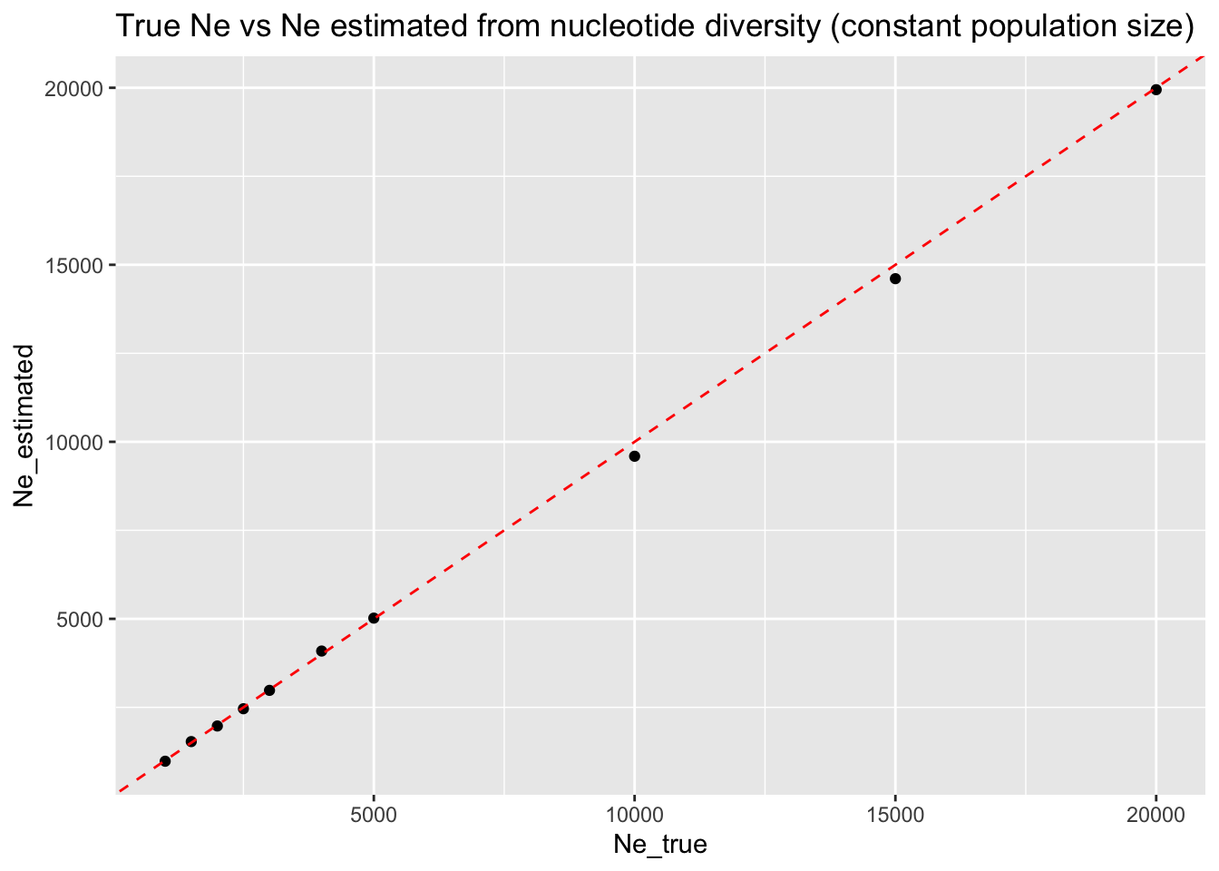
This toy exercise is a great example of how to use these kinds of simulations in practice. Again, nucleotide diverisity-based \(N_e\) estimation and its benchmarking across a range of parameters is only an example for demonstration, but this idea extends to many other settings:
benchmarking of IBD accuracy across different gene-flow scenarios,
validating qpAdm inference results for various possible admixture graphs,
testing the robustness of local ancestry inference methods (LAI) and admixture dating inference as a function of admixture times and proportions,
understanding how PCA differs for different sample sizes from different populations,
… and many others.
Exercise 6: Comparing multiple models
Let’s make it a bit more interesting and more practically relevant. Suppose we want to see how robust our estimator is to the assumptions behind the underlying demographic model (which is almost always uncertain to some degree, meaning that our assumptions can be also uncertain!).
In the previous exercise, we used nucleotide diversity to infer the \(N_e\) of a population under study (we used an equation, but it could be also external software) and verified that it works very well for a model of a constant population size.
But what about population that experienced a resize event? How well does our \(N_e\) estimate work in such case?
In your script slendr_Ne_pi.R, make a copy of your function sim_constant() and name that copy sim_change(). Make the following changes to this function:
the population “pop” will start with fixed \(N_e\) of 5000,
the population will experience a population resize (implemented by the function
resize()), which will set the size of the population to the value given to the argumentNe_trueat time 1000.
Then, use map_dfr() to run the new function sim_change() along the same parameter grid as before, visualizing the results of Ne_true against Ne_estimated again. How well does our diversity-based \(N_e\) estimate perform in such a demographic scenario? Is it robust to non-constant demographic histories? If not, why?
NoteClick to see the solution
Here’s the solution—new function sim_change(), new simulation run against a parameter grid, and a visualization of results:
# new function to simulate population size change
sim_change <- function(Ne_true) {
pop <-
population("pop", time = 2001, N = 5000) %>%
resize(N = Ne_true, time = 1000)
model <- compile_model(populations = pop, generation_time = 1, direction = "backward")
ts <-
  msprime(model, sequence_length = 10e6, recombination_rate = 1e-8) %>%
  ts_mutate(mutation_rate = 1e-8)
df <- ts_diversity(ts, list(all = ts_names(ts)))
df$Ne_estimated <- df$diversity / (4 * 1e-8)
df$Ne_true <- Ne_true
df
}
# simulations across a parameter grid
Ne_grid <- c(1000, 1500, 2000, 2500, 3000, 4000, 5000, 10000, 15000, 20000)
df_change <- map_dfr(Ne_grid, sim_change)
# visualization of results
ggplot(df_change, aes(Ne_true, Ne_estimated)) +
geom_point() +
geom_smooth(color = "red", linetype = "dashed") +
ggtitle("True Ne vs Ne estimated from nucleotide diversity (population size change)") +
xlim(0, 20000) +
ylim(0, 20000)`geom_smooth()` using method = 'loess' and formula = 'y ~ x'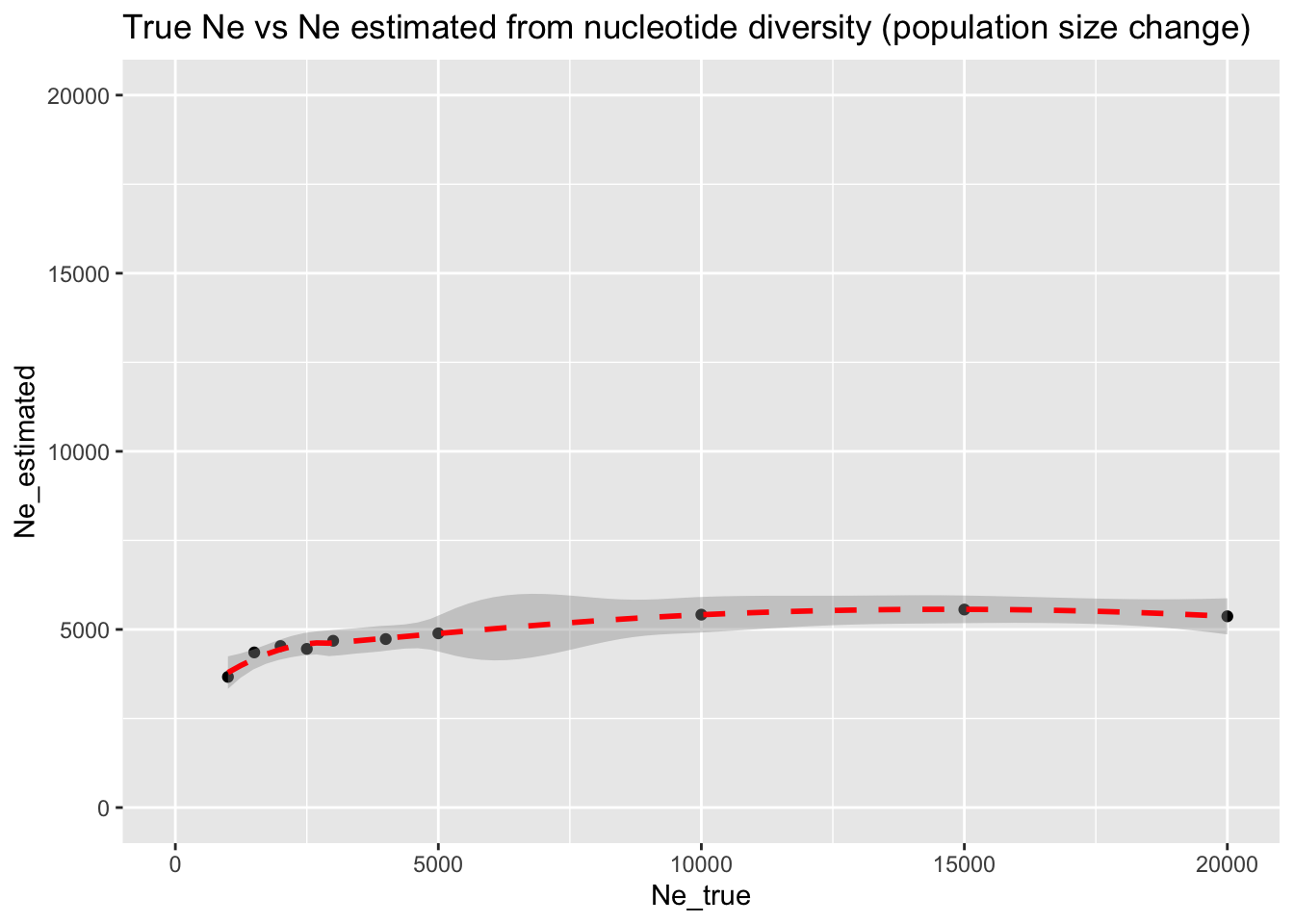
We can see that even a large population resize event doesn’t change the observed levels of nucleotide diversity that much. As a result, the \(N_e\) based on the population nucleotide diversity is very wrong—we consistently estimate it at the level of 5000 (i.e., the size prior to the resize), regardless of the true size of the population after the resize.
It’s only very drastic bottlenecks that are picked up by our \(N_e\) estimator, and even in those cases we still severely overestimate the true \(N_e\) after the resize event.
Exercise 7: Expanding the parameter grid
Our hypothesis for how poorly the nucleotide diversity-based estimate of \(N_e\) is doing under non-constant population size is that the resize event is very recent. As a result, diversity hasn’t yet reached an equilibrium value which would be picked up by our \(N_e\) estimator.
Let’s test this hypothesis while, at the same time, showing how we can expand the parameter grid simulations to include another parameter—this time the time of the population size change in addition to the \(N_e\) resize value.
In your script slendr_Ne_pi.R, add a second argument to your function sim_change() called T_change. Change the resize() command in your function to use variable T_change instead of the fixed value of 1000, then add another column called T_change to the data frame with the value of this argument before the function returns the results again. Then, run four versions of the map_dfr() command in the same way as before, except now in the form such as map_dfr(Ne_grid, sim_change, T_change = 100) (this will run sim_change() for each of the Ne_grid values like before, while fixing the T_change parameter to 100). Do this for T_change of 1, 100, 1000, and 2000.
When you visualize the results for each of the four simulation batches, do you see evidence supporting our hypothesis for why our \(N_e\) estimator performs poorly in sudden changes of \(N_e\)? And does the time since the resize change have an effect on the estimator as we hypothesized?
NoteClick to see the solution
Here’s the solution.
First, the new function sim_change() which now has two parameters Ne_true and T_change:
sim_change <- function(Ne_true, T_change) {
pop <-
population("pop", time = 2001, N = 5000) %>%
resize(N = Ne_true, time = T_change)
model <- compile_model(populations = pop, generation_time = 1, direction = "backward")
ts <-
msprime(model, sequence_length = 10e6, recombination_rate = 1e-8) %>%
ts_mutate(mutation_rate = 1e-8)
df <- ts_diversity(ts, list(all = ts_names(ts)))
df$Ne_estimated <- df$diversity / (4 * 1e-8)
df$Ne_true <- Ne_true
df$T_change <- T_change
df
}A new simulation run against a parameter grid (I’m rbind()-ing all four map_dfr() runs together because I want to use ggplot2 to visualize the results in a tidy way with four panels:
Ne_grid <- c(1000, 1500, 2000, 2500, 3000, 4000, 5000, 10000, 15000, 20000)

df_change <- rbind(
  map_dfr(Ne_grid, sim_change, T_change = 1),    # simulate size change 1 generation ago
  map_dfr(Ne_grid, sim_change, T_change = 100),  # simulate size change 100 generations ago
  map_dfr(Ne_grid, sim_change, T_change = 1000), # etc.
  map_dfr(Ne_grid, sim_change, T_change = 2000)
)
And finally, visualization of results:
ggplot(df_change, aes(Ne_true, Ne_estimated)) +
  geom_point() +
  geom_smooth(color = "red", linetype = "dashed") +
  ggtitle("True Ne vs Ne estimated from nucleotide diversity (population size change)",
          subtitle = "Each panel indicates the time of the population size change") +
  xlim(0, 20000) +
  ylim(0, 20000) +
  facet_wrap(~ T_change)
`geom_smooth()` using method = 'loess' and formula = 'y ~ x'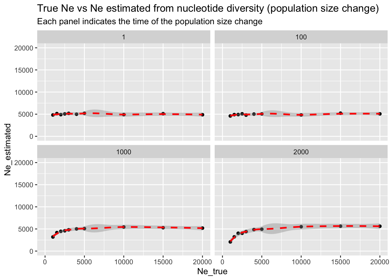
Here’s the same result, plotted in a single figure:
library(dplyr)

df_change %>%
  mutate(T_change = factor(T_change)) %>%
ggplot(aes(Ne_true, Ne_estimated, color = T_change, group = T_change)) +
  geom_point() +
  geom_smooth() +
  ggtitle("True Ne vs Ne estimated from nucleotide diversity (population size change)") +
  xlim(0, 20000)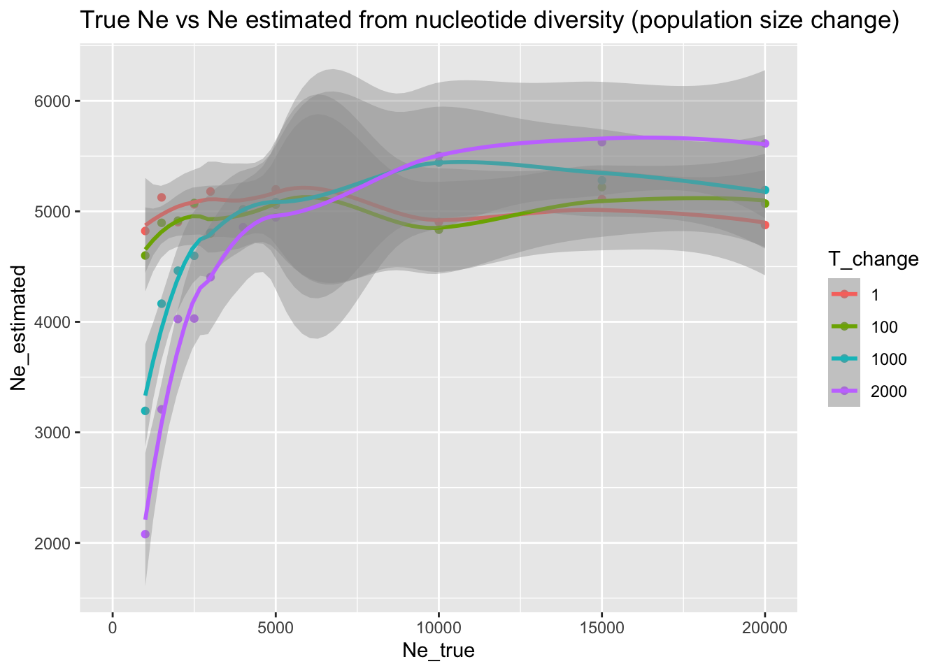
We can see that, indeed, the older the population resize event, the more time there’s for the population to lose genetic variation (in case of a bottleneck), or gain new variation (in case of population size increase—though we don’t really see the effect here), which means that the \(N_e\) estimated based on the \(\theta = 4 N_e \mu\) nucleotide diversity parameter is going to be a little closer to the true (unknown) population size.
Still, it’s absolutely clear that non-constant demography can completely mislead the \(N_e\) estimator based on nucleotide diversity—this is a conclusion that is actually quite relevant for real-world applications. For instance, we could have very endangered species (with a very small \(N_e\)) which still maintains quite a bit of nucleotide diversity!
In conclusion, the problem with the nucleotide diversity is that it effectively reduces the entirety of genetic variation in the population (which mutations there are at which frequencies) into a single number. As a result, we lose a lot of potentially very useful information about the population’s demographic history. When we try to estimate \(N_e\) using this summary statistic, we can only hope to infer a long-term \(N_e\), but we won’t be able to infer recent population dynamics.
As we have seen, a single bottleneck doesn’t cause nucleotide diversity to drop significantly enough for us to pick up that this bottleneck even happened.
Exercise 8: Real-world example
To put the simulation-based exploration above in a real-world context, let’s consider the case of estimating the \(N_e\) of a present-day modern human population.
Take a look at the Supplementary Table 1 published in this hugely influential paper. Look up the value of heterozygosity computed for the individual with the sample ID “S_Czech-2” in the column called “samtools autosomal heterozygosity”. What is the \(N_e\) value you can estimate from the heterozygosity observed in this individual, if you assume autosomal human mutation rate \(\mu\) of \(1.3 × 10^{−8}\) per base pair, per generation (1.3e-8 in R) and substitute the individual’s heterozygosity for the \(\theta\) parameter?
Knowing what you’ve learned from your simulation benchmarking of this simple \(N_e\) estimator above, how does your inferred modern human \(N_e\) fit in the context of the fact that there are more than 8 billion people in the world right now?
Bonus exercise: Allele frequency spectrum (AFS)
Create a new script called slendr_Ne_afs.R. Copy-paste the following code into that script. Note that this is the same exact model we started this chapter with (except for the one line which selects only 20 individuals from all individuals recorded in the tree sequence).
library(slendr)
init_env()

pop <- population("pop", time = 2001, N = 5000)
model <- compile_model(populations = pop, generation_time = 1, simulation_length = 1000)

ts <-
  msprime(model, sequence_length = 10e6, recombination_rate = 1e-8) %>%
  ts_mutate(mutation_rate = 1e-8)

subset <- sample(ts_names(ts), 10)
Unlike nucleotide diversity which, as mentioned above, reduces the entire genomic variation of a population into a single number, the allele frequency spectrum carries information about the distribution of the counts of mutations at each observable frequency.
Look at the ?ts_afs help page to learn how the slendr function ts_afs() works. As you’ve seen, ts_diversity() (like the vast majority of slendr statistical functions) produces a data frame. What data format does ts_afs() produce? Compute the AFS from your simulated tree sequence ts on your subset of individuals, then visualize it (with whatever means you know).
NoteClick to see the solution
As we can see, ts_afs() produces a plain R vector of integer numbers, each of which represents the count of mutations observed at a given frequency — the count of singletons, the count of doubletons, etc.:
afs <- ts_afs(ts, sample_sets = list(subset))
afs
[1] 12369 1871 1030 689 503 392 315 325 217 269 227 173
[13] 151 158 133 126 134 153 77 102 114This vector can be easily visualized with a base-R function plot():
plot(afs, type = "l", col = "lightblue", xlab = "allele frequency", ylab = "count")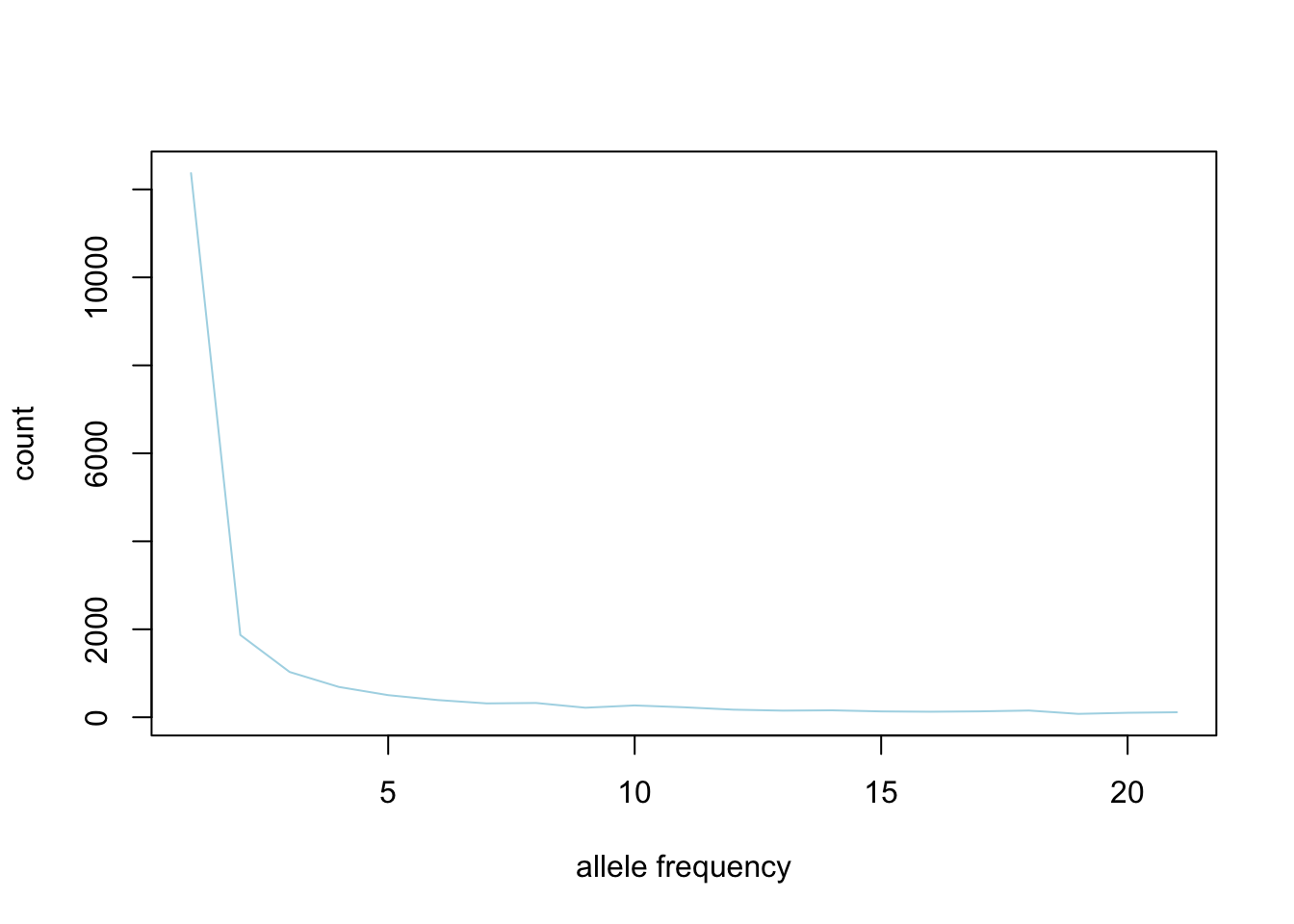
But does the AFS really carry more information about demographic changes?
Write a new function in your script, called sim_afs(), which will again accept a single argument Ne_true and implement the exact same demographic model as you did in your function sim_change() (i.e., resize from the initial N of 5000 to the given value of Ne_true at time 1000). In this function, compute the afs vector from this model, then run it for a range of Ne_grid values and visualize the individual AFS vectors produced for each of them. Does AFS pick up signal even from such recent population size changes, unlike the nucleotide diversity?
NoteClick to see the solution
Here’s a function which simulates an AFS for a demographic history given by the Ne_true argument:
library(ggplot2)
library(purrr)
library(dplyr)

library(slendr)
init_env()

sim_afs <- function(Ne_true) {
  pop <- population("pop", time = 2001, N = 5000) %>% resize(N = Ne_true, time = 1000)

  model <- compile_model(populations = pop, generation_time = 1, direction = "backward")

  ts <-
    msprime(model, sequence_length = 10e6, recombination_rate = 1e-8) %>%
    ts_mutate(mutation_rate = 1e-8)

  subset <- sample(ts_names(ts), 10)

  afs <- ts_afs(ts, sample_sets = list(subset))

  # return the result not as a plain integer vector, but a proper data frame
  # annotated by the frequency bin number -- this makes visualization of
  # results later with ggplot2 much easier
  data.frame(
    Ne_true = Ne_true,
    frequency = 1:length(afs),
    count = afs
  )
}
We run the AFS simulation batch in the same way as we did before:
df_afs <- map_dfr(Ne_grid, sim_afs)And we visualize the individual AFS vectors, colored by their underlying assumed \(N_e\) after the demographic history change:
ggplot(df_afs, aes(frequency, count, color = factor(Ne_true))) +
  geom_line() +
  ggtitle("AFS vector for different population size change models")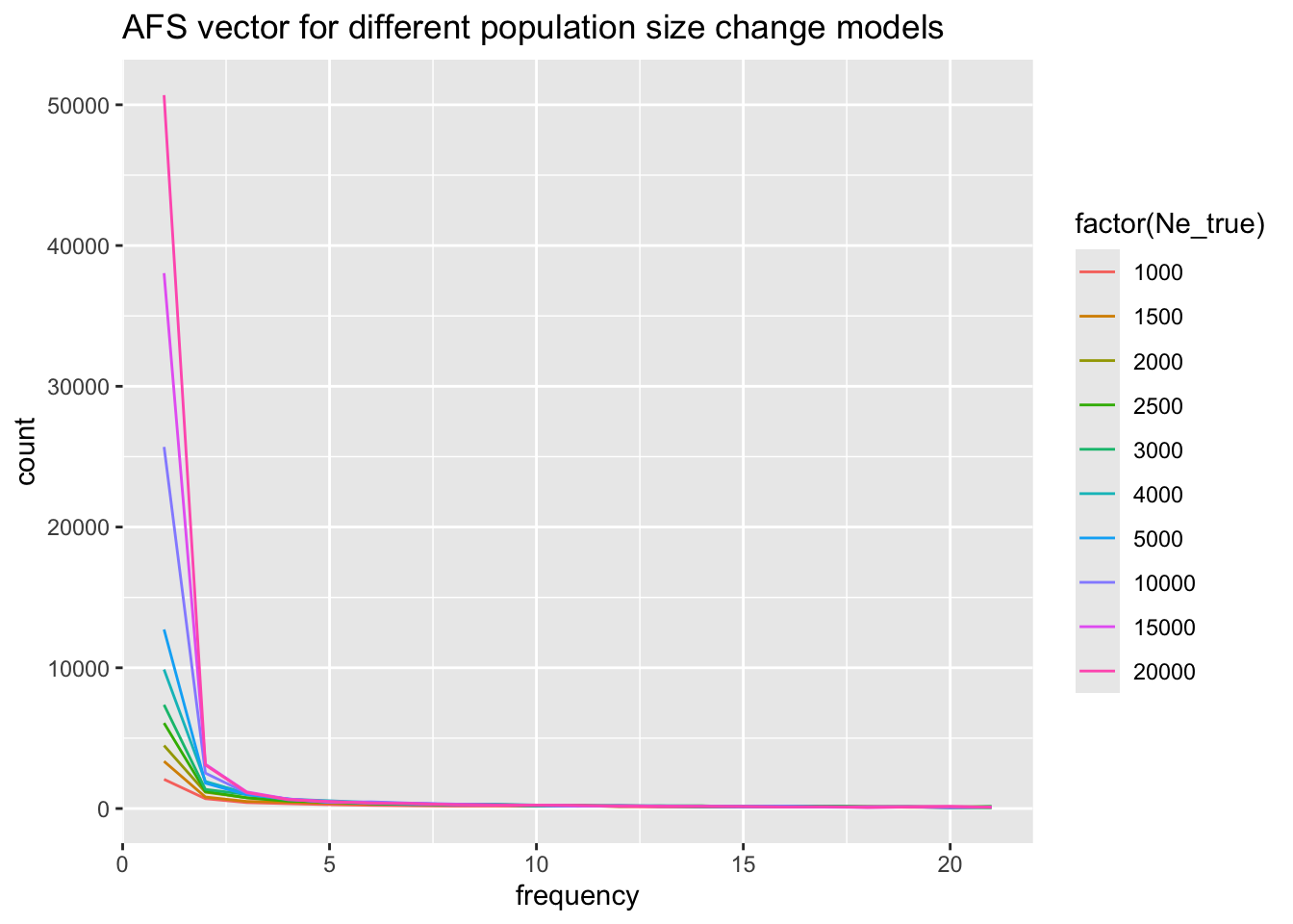
For easier comparison, here are the AFS result side-by-side with the values of nucleotide diversity from the same demographic scenarios:
`geom_smooth()` using method = 'loess' and formula = 'y ~ x'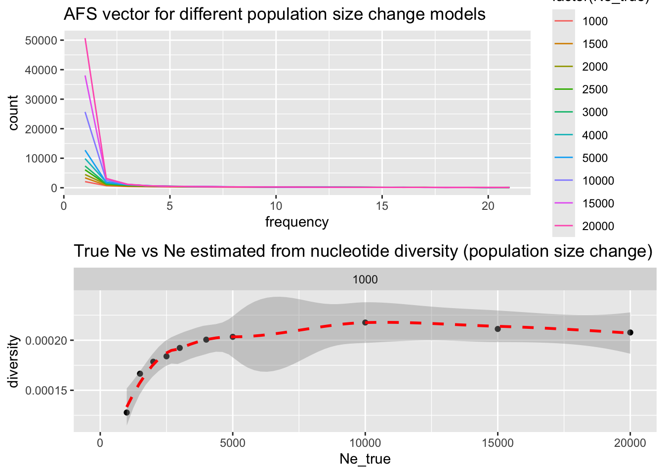
This simulation indicates that AFS does, indeed, carry much more information about population history, even for recent changes in population size, driven largely by singletons! Therefore, at least for population expansions, AFS is much more statistically powerful than nucleotide diversity. From population genetic theory perspective this makes sense, because nucleotide diversity is actually nothing but a summary of the AFS.
For now we’ll leave this topic be. We could go much deeper into this, but the point of this chapter was to demonstrate how to compute within-population statistics with slendr, how we can use manipulation of R lists and vectors to instruct slendr on how to compute a given statistic, and provide a set of small examples of how population genomic simulations (even extremely simple ones!) and a bit of data processing can be used to benchmark real-world inference methods..
Towards the end of the workshop, you’ll have the opportunity work through a slightly more realistic case-study which will demonstrate how to do simulation-based inference of \(N_e\) in a fully automated way.
Catching up
Here is a complete solution to the exercises in this section represented by a single tidy reproducible R script: