library(slendr)
init_env()Building slendr models
Theme of this chapter
What features does slendr offer for encoding traditional demographic models (i.e., tree-like models featuring population splits, population size changes, and admixture)? How can we transform a model that came up in a discussion, in a brainstorming session, or which we saw in a figure in a research paper, into a working script as quickly as possible?
Preparation
A couple of points before we start this chapter.
- Every one of your solutions for each exercise should contain the following two lines of code. If you get errors about missing functions, simulation failures, etc., make sure your script isn’t missing this little bit of code.
Or, alternatively, this (depending on how the slendr Python environment is set up):
library(slendr)
init_env(uv = TRUE)- Try to write your solutions in a dedicated script (saved under an appropriate name) as instructed by any given exercise. Don’t write everything into a single long file, or only in your R console (without having things recorded in a dedicated solution script).
The second point might be frustrating at times and appear like unnecessary extra work, but keeping your code organized (and also annotated with # comments like this) is critical for making your computational workflows reproducible.
Exercise 1: Forward direction of time
Create a new R script and save it as forward_model.R. Write your solutions to this exercise into that script.
Encode the demographic model sketched in the following diagram using a series of population() calls, then compile it with compile_model(), storing it in the model variable (it should be compiled to run for 401 generations total with the generation time of 1). Finally, verify the correctness of the model visually using using the function plot_model(). Make sure to write all of this code in your script forward_model.R
Hint: Try to get into the habit of executing each command you add to your script (a line of code, a couple of lines, etc.) in your R console by pressing Ctrl+Enter as you’re writing your solutions line by line.
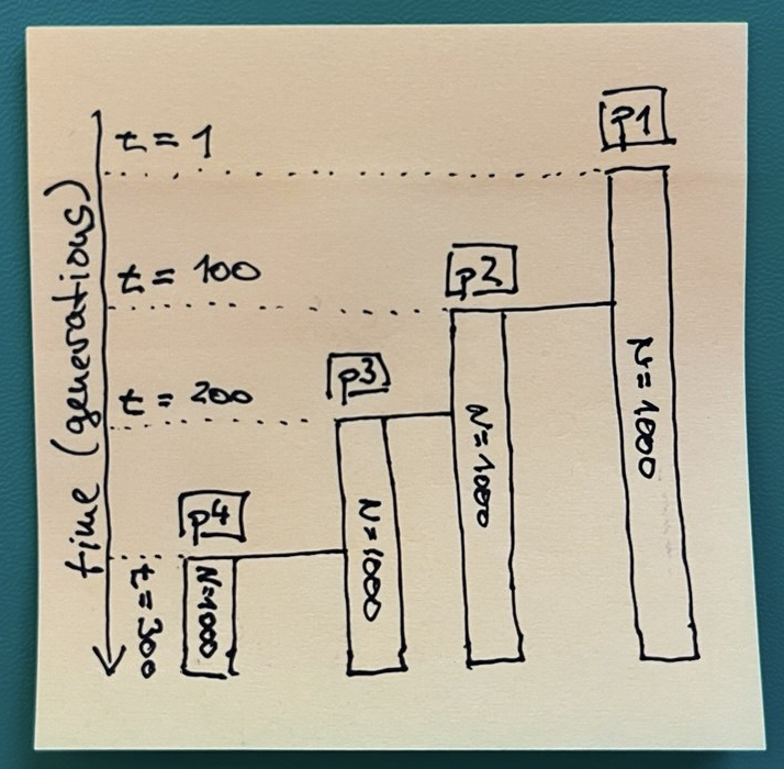
Note: At this moment, the time value has a completely arbitrary unit to be determined later. Additionally, unless otherwise specified, the size N will always indicate the “effective population size” \(N_e\).
NoteClick to see the solution
As always, we start our new script by loading slendr itself and activating its environment:
library(slendr)
init_env()
Adding to the script, we begin by creating the first population, called “p1”, storing it in a variable with the same name. When we execute this line and type p1 in the R console, we get an informative summary. Especially when building very complex models with slendr, it pays off to develop the habit to program models like this, one command at a time, always making sure that what we are programming matches what we want to program!
p1 <- population("p1", time = 1, N = 1000)

p1
slendr 'population' object
--------------------------
name: p1
non-spatial population
stays until the end of the simulation
population history overview:
- time 1: created as an ancestral population (N = 1000)Here is, then, the complete solution:
library(slendr)
init_env()

p1 <- population("p1", time = 1, N = 1000)
p2 <- population("p2", time = 100, N = 1000, parent = p1)
p3 <- population("p3", time = 200, N = 1000, parent = p2)
p4 <- population("p4", time = 300, N = 1000, parent = p3)

model <- compile_model(populations = list(p1, p2, p3, p4), generation_time = 1, simulation_length = 401)

plot_model(model)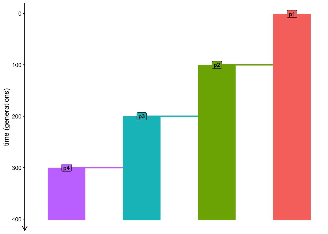
What happens when you don’t specify the simulation_length argument of the compile_model() function? Try running your compile_model() command without this argument. Do you get an error if you leave out this argument? Why?
Exercise 2: Backward direction of time
Unlike most other simulation frameworks (which all use either forward or backward time direction, but never both), slendr gives us a lot of flexibility in how to encode the time units of our models, or even the direction of time used by our models. This saves us costly (and error-prone) conversion of model time units appropriate for our concrete use-case.
Create a new R script and saved it as backward_model.R. Write your solutions to this exercise into that script.
Convert the forward model which you just wrote into using a backward direction of time (i.e., the model will implicitly end at time 0—“the present day”—and start at the appropriate “time ago”). You can start by copying the contents of forward_model.R into your new script, and modify it as needed. Again, visualize the final model using the plot_model() function, which should get you (visually) exactly the same figure.
NoteClick to see the solution
To solve this exercise, we simply have to take the total length of our original forward simulation and reverse the times of scheduled events accordingly.
Note that this is very annoying to do (and I’m sorry I’m making you do frustrating stuff!). This is just to show what’s necessary to do with simulation frameworks other than slendr. This convenient flexibility becomes even more clear once we start dealing with realistic time units later.
For now, just remember that the direction of time of our models in slendr is flexible:
If you want to simulate yeast growing over generations in a lab (starting from generation 1), you can.
If you want to simulate human history over thousands of years (starting, for instance, from the Anatolian migration thousands of years ago), you can.
Here’s a complete solution for the backward-time model:
library(slendr)
init_env()

p1 <- population("p1", time = 400, N = 1000)
p2 <- population("p2", time = 300, N = 1000, parent = p1)
p3 <- population("p3", time = 200, N = 1000, parent = p2)
p4 <- population("p4", time = 100, N = 1000, parent = p3)

model <- compile_model(populations = list(p1, p2, p3, p4), generation_time = 1)

plot_model(model)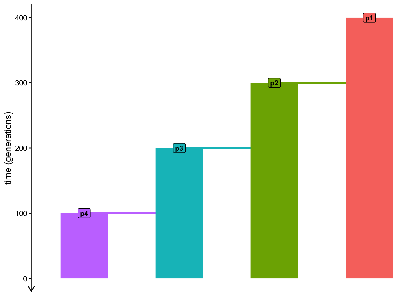
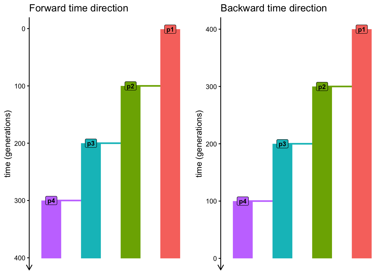
Indeed, when we compare both figures side by side, we see that the forward and backward versions of the two model give the same figure (except for the “direction” of time units along the y-axis):
In the previous exercise, leaving out the simulation_length argument resulted in an error. Do you get an error when you leave it out this time, for the backwards-time model? Why? Or why not?
In your backwards model, what happens when you set simulation_length to a number that is shorter than the intended duration of the model in the sketch at the beginning, like setting simulation_length = 120? What would this imply about our programmed model? Do this only in your R console, you don’t have to modify your script permanently. This is just a demonstration of an occasionally useful feature of slendr.
NoteClick to see the solution
If we do set the argument to a smaller number, we effectively “truncate” the duration of the model. This is arelatively rare thing to do, but it could be useful in some circumstances so it’s worth mentioning here:
model <- compile_model(
  populations = list(p1, p2, p3, p4),
  generation_time = 1,
  simulation_length = 120
)

plot_model(model)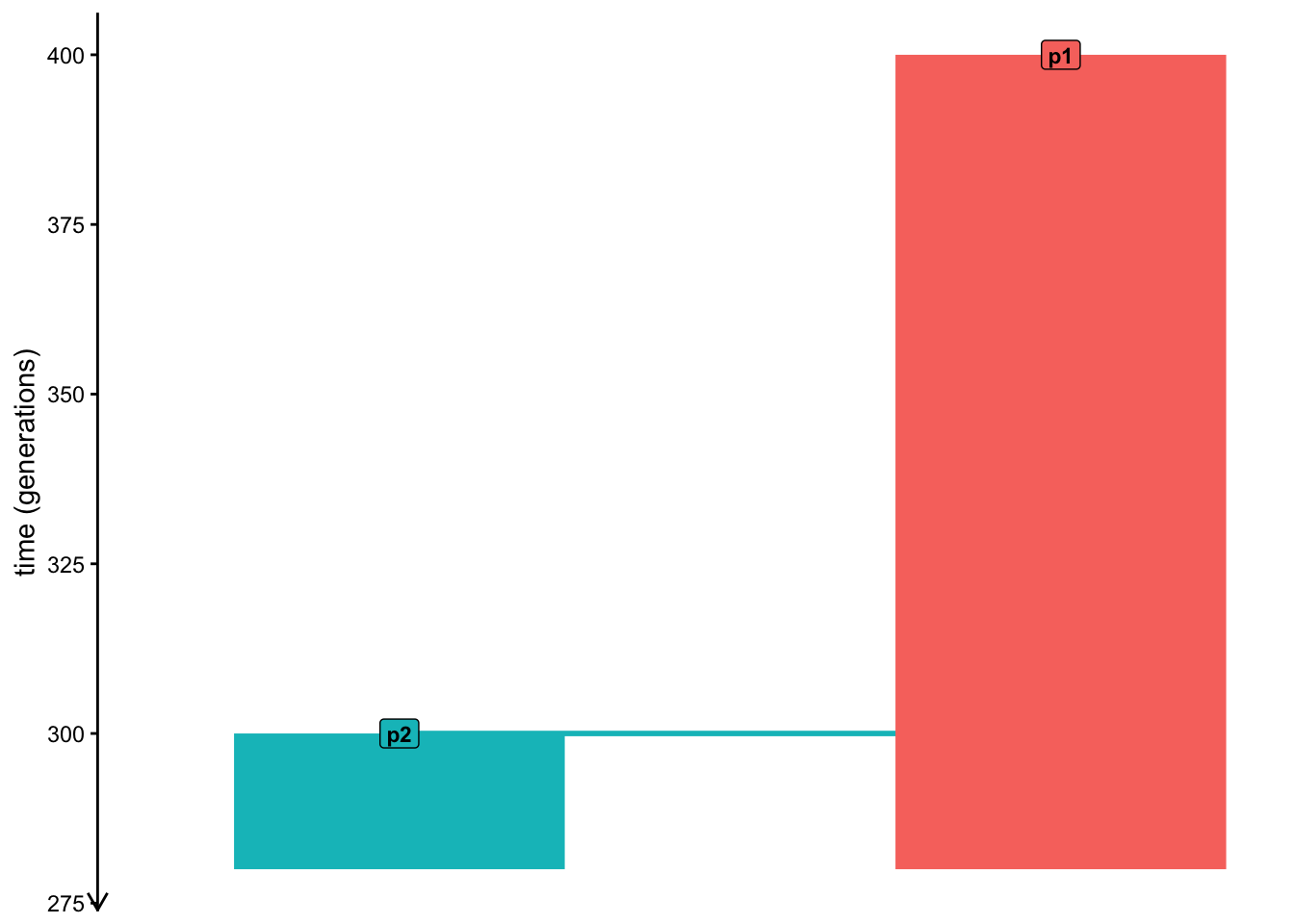
We can again compare the two models side by side to see the truncation more clearly:
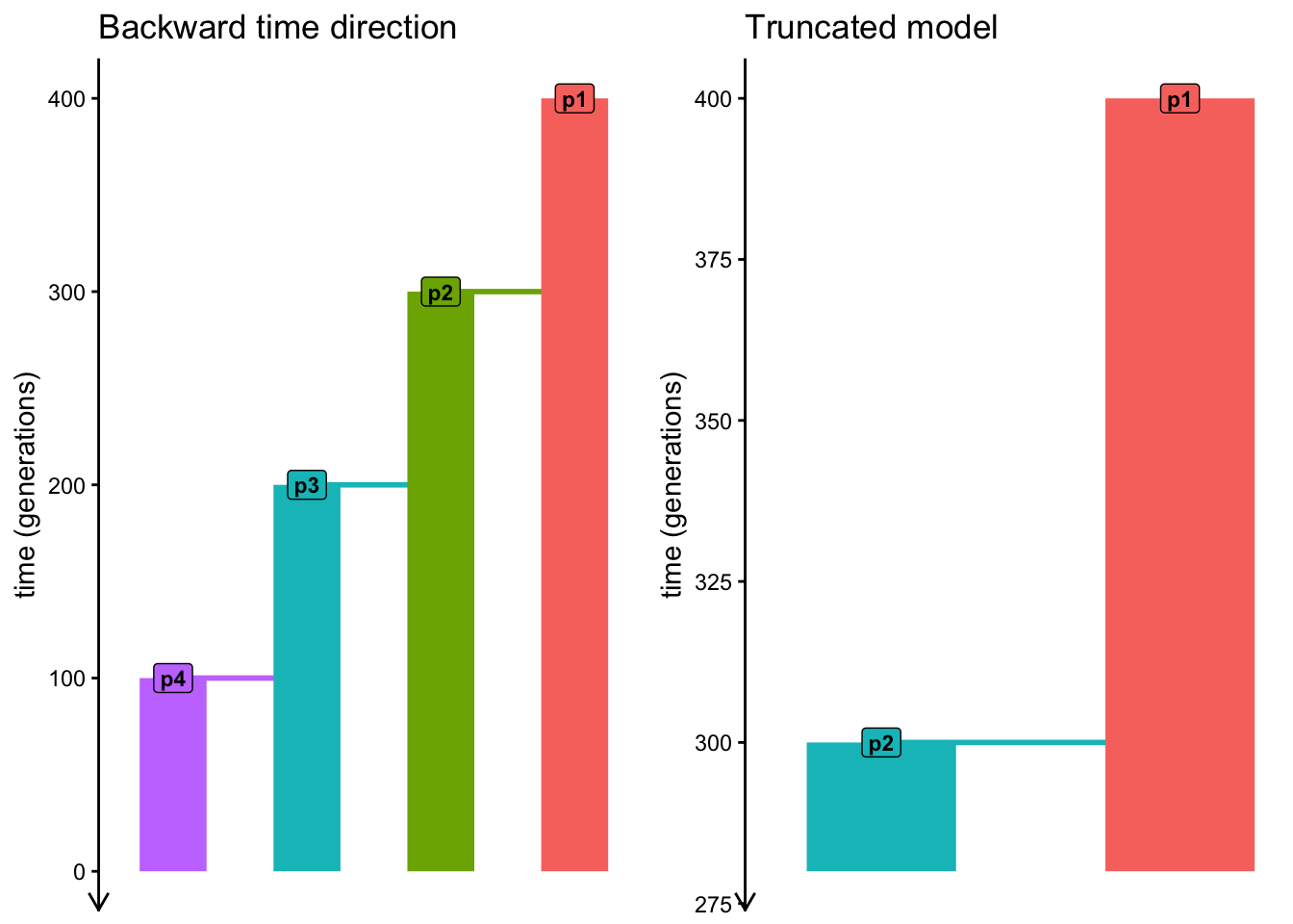
Fun fact: I discovered a bug in slendr when I was writing this exercise. I had to write an emergency bugfix just in time for the workshop, but I’m just now realizing that I got the color scheme wrong. Sorry about that! To be fixed later (on my TODO list already).
Exercise 3: Custom time units
For theoretical models, encoding time in generations is generally enough. However, in more empirical settings, encoding times in other units can be quite handy. For instance, imagine you work with ancient DNA samples assigned with radiocarbon dates which use units of “years before the present”. Having to manually convert such times into generations gets cumbersome quickly, both when programming models and when analyzing simulated sequence data.
This is where the generation_time argument of compile_model() comes into the picture—with this argument, we instruct slendr on how should the “generic time numbers” in our model code interpreted as “real-world numbers”. Additionally, there’s another optional argument called time_units which we can use to give the numbers an explicit description.
Create a new script human_model.R and copy your current contents of backward_model.R into it. Then change your code so that the time units can be interpreted as “years before present (BP)”, using the approximate human generation time of 30 years per generation. Finally, visualize the model to make sure you’ve programmed everything correctly (perhaps by comparing the visualization to that of the previous forward and backward models).
Hint: This may sound more complicated than it is. Basically, you want to modify the times of all demographic events in your model—originally in units of generations—so that they are effectively 30-times larger (so that the times represent human generation times), and make them run from larger values to smaller values (so that they represent times “years before present (BP)” or “years ago”). Finally, for clarity, you might want to use the time_units argument of compile_model() to give the units this exact description.
NoteClick to see the solution
Here’s the original model transformed into what could represent “human demography” (particularly because all times are now in units of “years ago”, and populations assumed to have the generation time of 30 years):
library(slendr)
init_env()

p1 <- population("p1", time = 12000, N = 1000)
p2 <- population("p2", time = 9000, N = 1000, parent = p1)
p3 <- population("p3", time = 6000, N = 1000, parent = p2)
p4 <- population("p4", time = 3000, N = 1000, parent = p3)

model <- compile_model(
  populations = list(p1, p2, p3, p4),
  generation_time = 30,
  time_units = "years before present"
)

plot_model(model)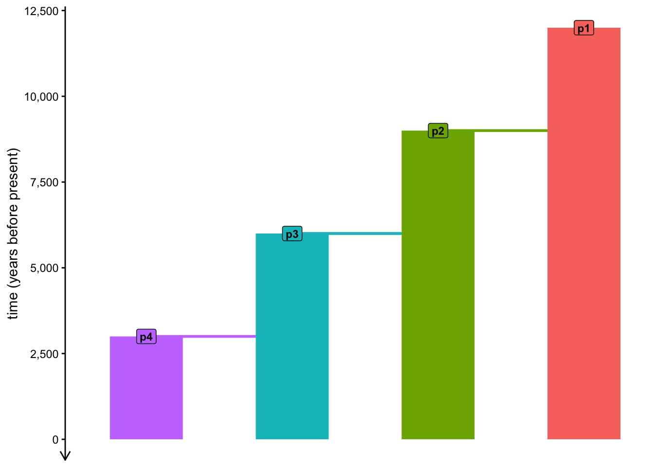
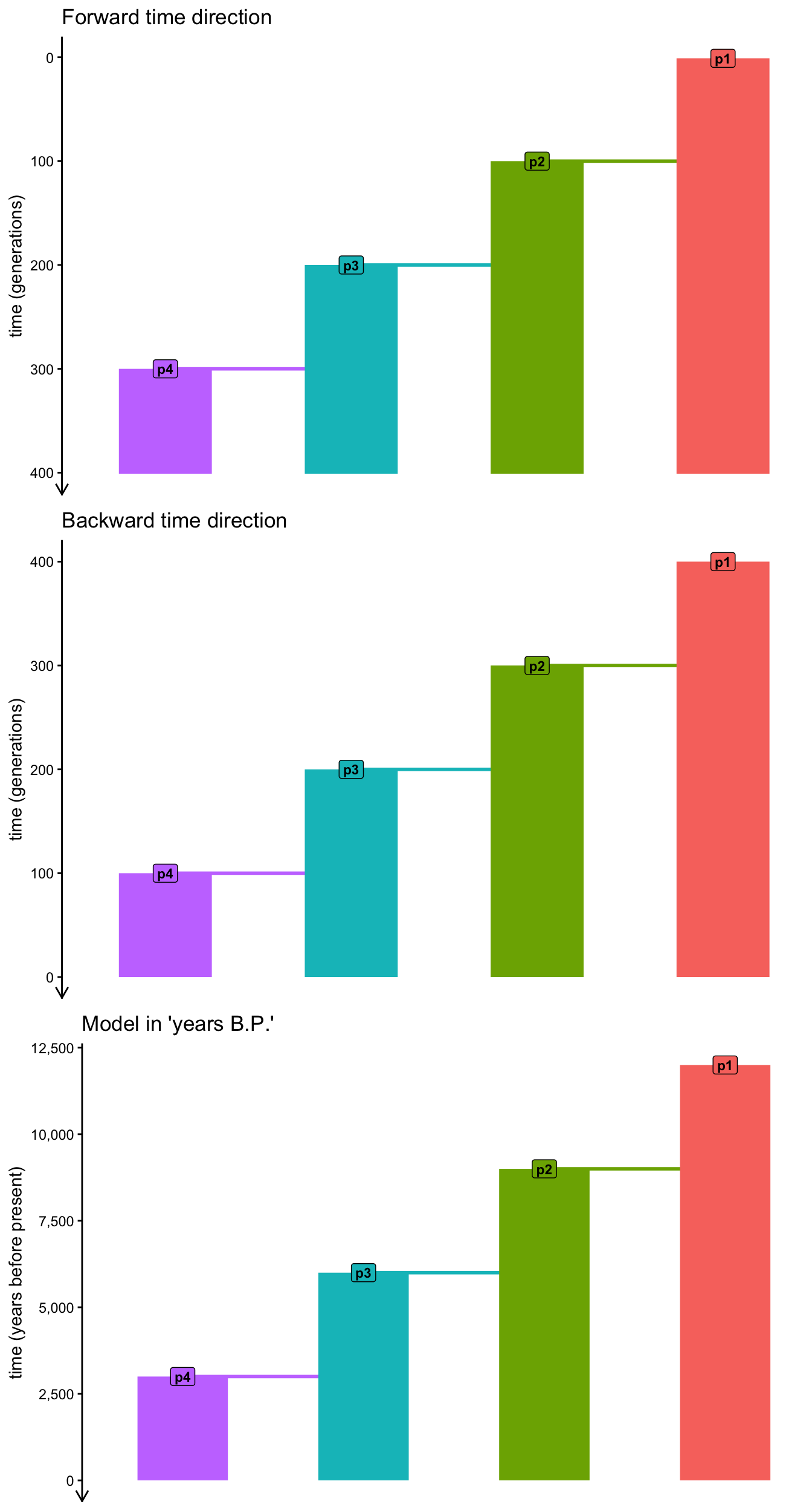
Again, when we compare this model to the very first model (which used time units of generations running forward in time), we see that they are completely identical—only the presentation changes (making the model more convenient for a reader expecting human demography), but the population genetics theory underlying this model remains the same!
Exercise 4: Programming gene flow
Of course, real-world populations don’t just split from one another. Another common demographic process is gene flow (also called admixture or introgression in various contexts and in different species).
Modify your human_model.R script, adding a command to program admixture from population p2 into population p3 starting at time 3000 “years ago”, with an end at time 2100 “years ago”, using the function gene_flow(). Set the total proportion of the p2 ancestry in p3 at 0.1 (i.e., 10% of the final p3 population will be derived from p2). When you plot this model using plot_model() (set also proportions = TRUE), you should see your “population tree model” turned into an “admixture model” (as these models are often called in the literature) with an arrow indicating the programmed admixture event.
NoteClick to see the solution
Here’s the current status of human_model.R, now featuring an admixture event:
library(slendr)
init_env()

p1 <- population("p1", time = 12000, N = 1000)
p2 <- population("p2", time = 9000, N = 1000, parent = p1)
p3 <- population("p3", time = 6000, N = 1000, parent = p2)
p4 <- population("p4", time = 3000, N = 1000, parent = p3)

gf <- gene_flow(from = p2, to = p3, start = 3000, end = 2100, proportion = 0.1)

model <- compile_model(
    populations = list(p1, p2, p3, p4),
    gene_flow = gf,
    generation_time = 30,
    time_units = "years before present"
)

plot_model(model, proportions = TRUE)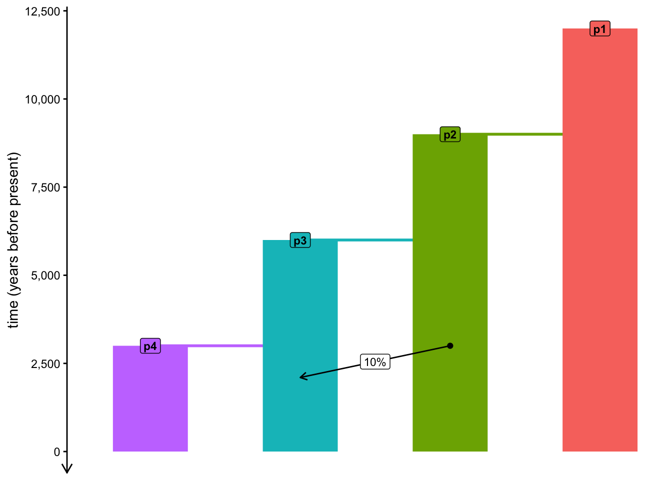
When you look at the ?gene_flow help page, you can see that the function has a migration_rate argument. What does it do? Is there any way to get the same result (i.e., to encode the same 10% ancestry gene-flow event) as you did just above, but using rate instead of proportion? When would you expect to use one or the other?
Hint: Try to make the habit of reading the help of various functions frequently—you discover lots of useful information that way that you wouldn’t normally learn about.
NoteClick to see the solution
A 10% proportion of p2 ancestry derived from p3 over the time window of 3000 to 2100 years ago is mathematically equivalent to a per-year rate of 0.1 / (3000 - 2100), i.e. ~0.000111. To express this in a slendr model, take a look at the modified call to gene_flow() below:
library(slendr)
init_env()

p1 <- population("p1", time = 12000, N = 1000)
p2 <- population("p2", time = 9000, N = 1000, parent = p1)
p3 <- population("p3", time = 6000, N = 1000, parent = p2)
p4 <- population("p4", time = 3000, N = 1000, parent = p3)

# same gene-flow event, now expressed as "yearly migration rate" instead of
# the "total admixture proportion" as before
year_rate <- 0.1 / (3000 - 2100)
gf <- gene_flow(from = p2, to = p3, start = 3000, end = 2100, migration_rate = year_rate)

model <- compile_model(
    populations = list(p1, p2, p3, p4), gene_flow = gf,
    generation_time = 30,
    time_units = "years before present"
)

plot_model(model, proportions = TRUE)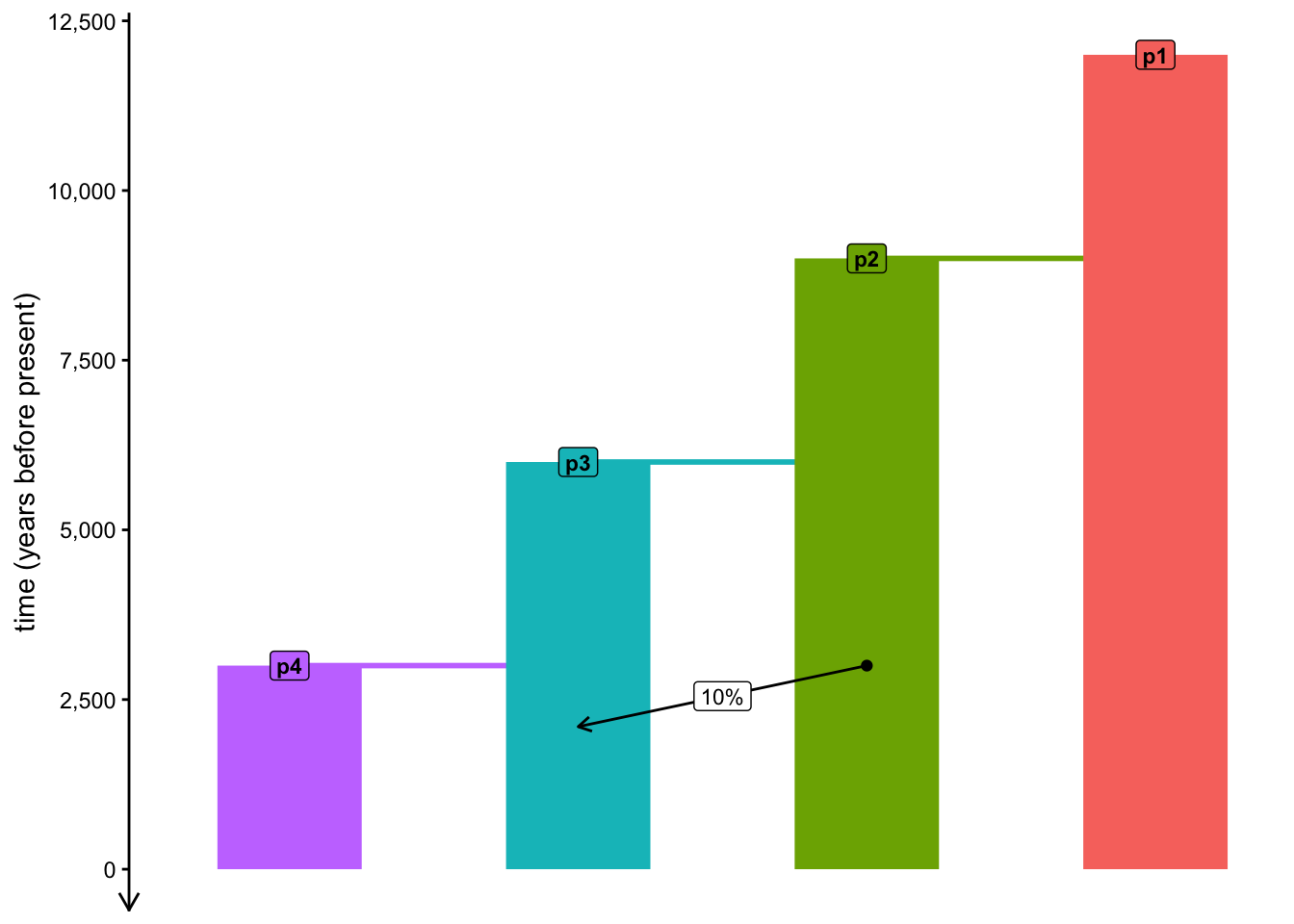
This is useful because sometimes we need to model a situation such as “we expect this number of migrants arriving into this settlement per generation” etc., in which case we don’t necessarily know the total proportion of genetic ancestry which would arrive like this in aggregate.
Exercise 5: Deciphering common errors produced by slendr
slendr is designed around interactive use, executing little bits of code at a time, making sure that potential errors are caught as soon as we make them rather than after spending lots of time programming long (and potentially eventually broken) simulation scripts.
However, software errors often confuse new programmers, especially because most errors represent completely trivial typos and unintended mistakes rather than conceptual issues with the model logic. Situations when “basically correct script” still gives errors are incredibly frustrating.
This is why it’s a good idea to spend a few moments to study the most common errors in slendr and recognize why they occur in an isolated, controlled setting when done on purpose.
First, let’s do a bit of a setup using things you already know. Create a new slendr model script called slendr_errors.R, just to have a “throwaway script” to experiment in without breaking your other working code.
Create an R variable pop containing a slendr population (using the population() function) with the name “pA”, at time 1 and with \(N_e\) of 5000. Then, create a population “pB” of the same size, which splits from “pA” at time 100. Then run this tiny toy script in your R console.
When slendr runs this code, it automatically infers that you intend to specify time in your model flowing in the forward direction (because times of your events move from smaller numbers to larger numbers). Not only that, from this point on, slendr will also enforce all following demographic events to follow this time direction!
To see how this works, create a third population named “pC”, which splits from pB at time 80. What does slendr do when you re-run your (now three-population) script? What error do you get? And if you were to fix this error, what’s the closest appropriate value of the pC split time from pB which would be consistent with slendr’s assumptions outlined above (and so it wouldn’t complain anymore)?
NoteClick to see the solution
We get an error because in the context of the model so far (pA starting at time 1 and pB splitting from it at time 100), pC would effectively split at an earlier time than it’s parent!
pC <- population("pC", time = 80, N = 5000, parent = pB)Error:
! The model implies forward time direction but the specified split
time (80) is lower or equal to the parent's (100)We can see that even setting the split time of pC to time 100 doesn’t work, because slendr enforces that a population can only split from its parent population at the time the latter already exists in the model:
pC <- population("pC", time = 100, N = 5000, parent = pB)Error:
! The model implies forward time direction but the specified split
time (100) is lower or equal to the parent's (100)In other words, the earliest that pC can split is time 101:
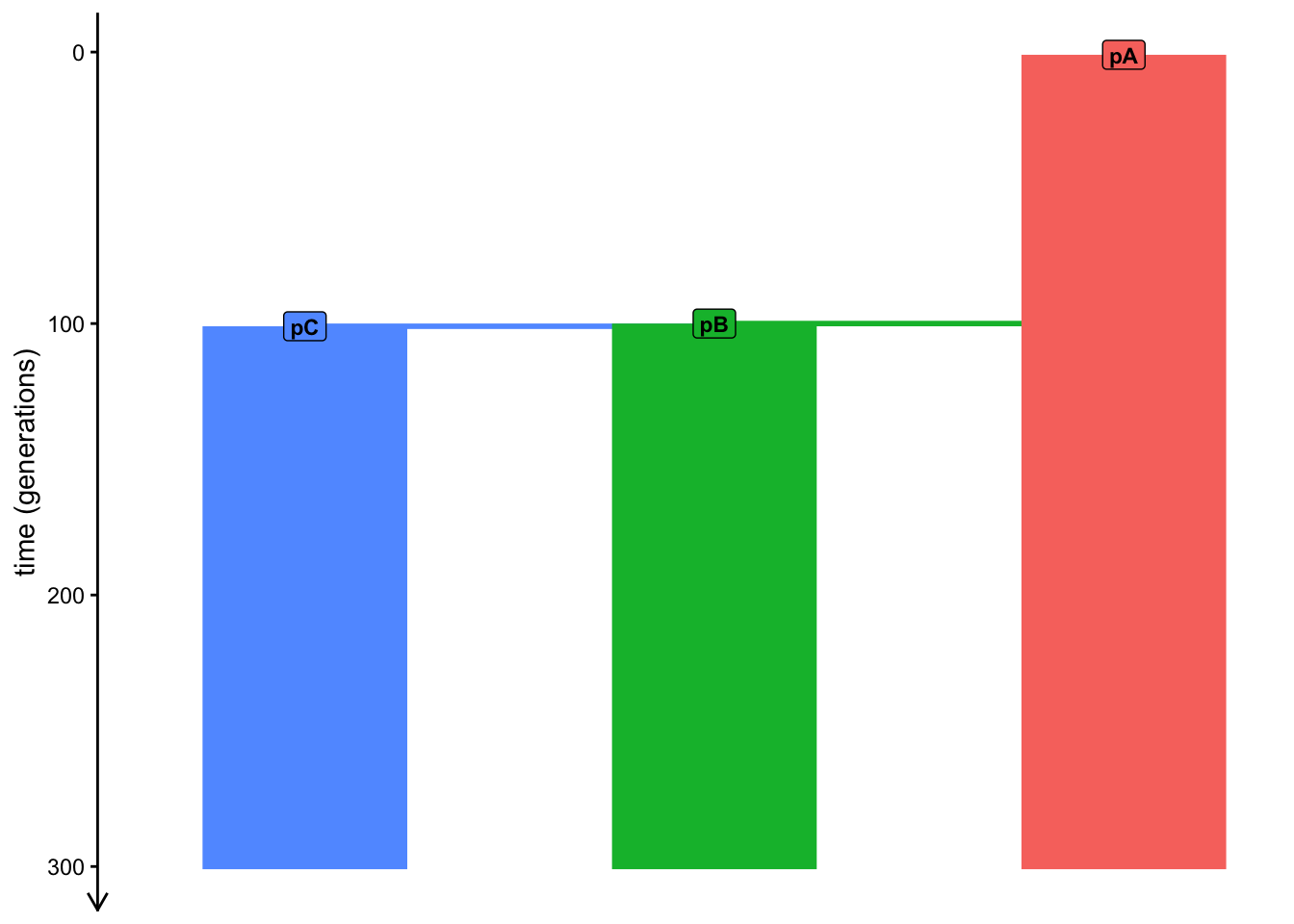
pC <- population("pC", time = 101, N = 5000, parent = pB)Giving us this model (we can barely see the difference between pB and pC splits because they’re separated by only 1 generation difference in time):
As another example, let’s look at gene_flow(), which programs gene flow between two populations represented by two R variables. Let’s say that (still in your script slendr_errors.R) you try to program:
42% gene flow from
pAtopCstarting at time 200 and ending at time 150, orgene flow starting at time 150 and ending at time 200.
Which of those two calls to gene_flow() do you think will result in an error and why? Try to answer this first before you actually run any of these two gene_flow() commands, then verify your intuition by executing those commands. As a help, you may want to visualize a compiled version of this model using plot_model() (or just look at this visualization in my solution to the previous exercise).
Note: There are other cases in which even the enforcement of model consistency described above still allows broken models to be programmed, which is why compile_model() provides yet another set of sanity checks. But we will leave those aside for now. If you end up running into these issues, this exercise has already equipped you to understand why slendr sometimes gives errors and how to interpret them to fix your models. And if in doubt, you can always ask me!
Exercise 6: Resize events
Finally, populations in traditional demographic models don’t just split and mix—they also experience population bottlenecks, population expansions, contractions, etc. The means to program these demographic events is through the function resize().
In slendr, these events come in two variants, which we can call step resizes or exponential resizes.
- Step resizes
We can implement immediate step resize events simply by calling the function resize(), providing the new size N for the population and the time at which the resize event should occur.
- Exponential resizes
If we need to implement exponential resize event (either exponential increase or decrease of population size), we provide the new size N, the time at which the resizing should start (same as for step resizes) but also the time at which it should end. From this information, slendr is able to interpolate the resizes needed at each time point in order to simulate the gradual exponential change.
Let’s get back to our script human_model.R. Practice the application of the resize() function by programming a bottleneck event in the history of the population p3. The bottleneck should happen at 1800 years ago, with the population contracting to the size of 100 individuals. Then program a recovery of this population, resizing it in a step to size of 2000 individual at time 1000 years ago. Again, always use the function plot_model() to visualize your compiled model and validate that you’ve programmed the bottleneck scenario correctly.
NoteClick to see the solution
Here’s the complete human_model.R in its current state after implementing the bottleneck and recovery of p3:
library(slendr)
init_env()

p1 <- population("p1", time = 12000, N = 1000)
p2 <- population("p2", time = 9000, N = 1000, parent = p1)
p3 <- population("p3", time = 6000, N = 1000, parent = p2) %>%
  resize(N = 100, time = 1800) %>%
  resize(N = 2000, time = 1000)
p4 <- population("p4", time = 3000, N = 1000, parent = p3)

gf <- gene_flow(from = p2, to = p3, start = 3000, end = 2100, proportion = 0.1)

model <- compile_model(
  populations = list(p1, p2, p3, p4),
  gene_flow = gf,
  generation_time = 30,
  time_units = "years before present"
)

plot_model(model, proportion = TRUE)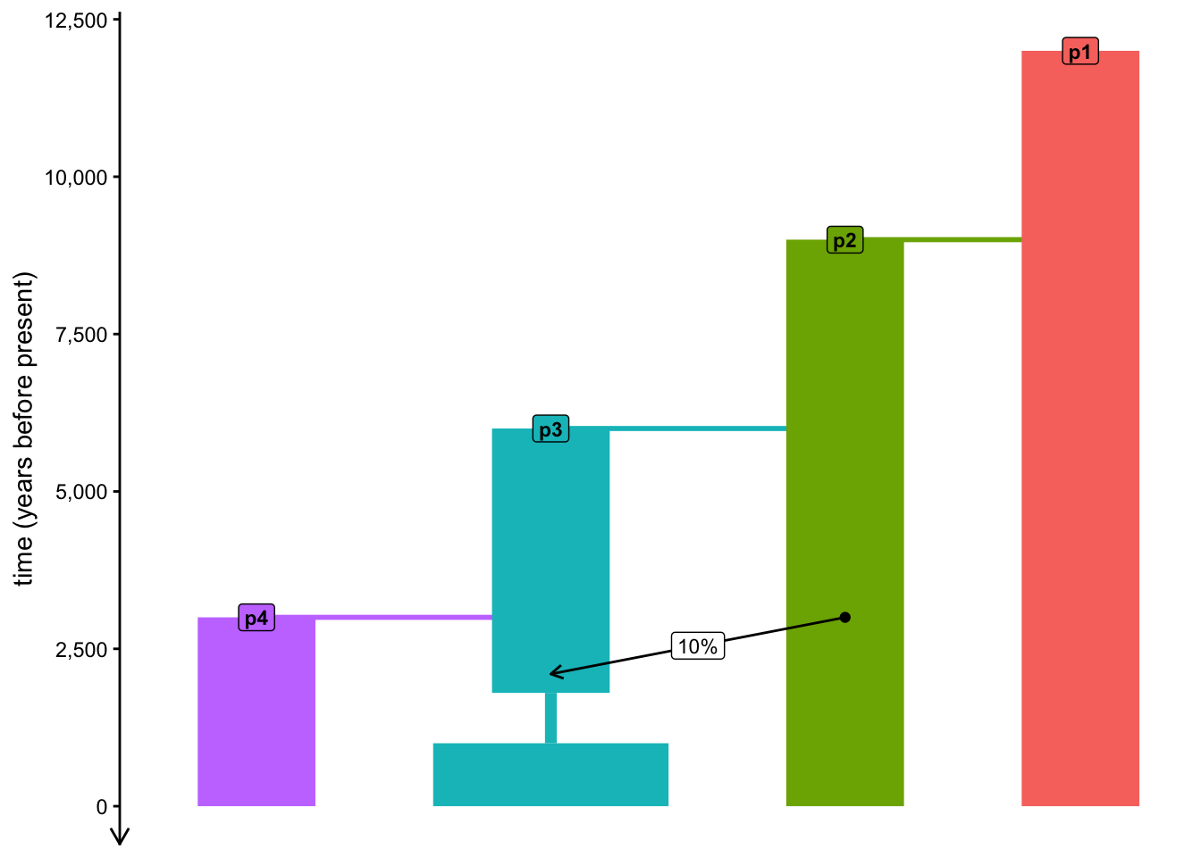
Note: The visualization of the exponential is a bit wonky in that it makes things look like a gradual linear change—apologies for that! This will be fixed in a future slendr version.
Catching up
If you want to just catch up to the point at which this chapter would conclude, here is the version of our simulation script human_model.R at the end of the final exercise:
NoteClick to see the script
human_model.R
library(slendr)
init_env()

p1 <- population("p1", time = 12000, N = 1000)
p2 <- population("p2", time = 9000, N = 1000, parent = p1)
p3 <- population("p3", time = 6000, N = 1000, parent = p2) %>%
  resize(N = 100, time = 1800) %>%
  resize(N = 2000, time = 1000)
p4 <- population("p4", time = 3000, N = 1000, parent = p3)

gf <- gene_flow(from = p2, to = p3, start = 3000, end = 2100, proportion = 0.1)

model <- compile_model(
    populations = list(p1, p2, p3, p4), gene_flow = gf,
    generation_time = 30,
    time_units = "years before present"
)

plot_model(model, proportions = TRUE)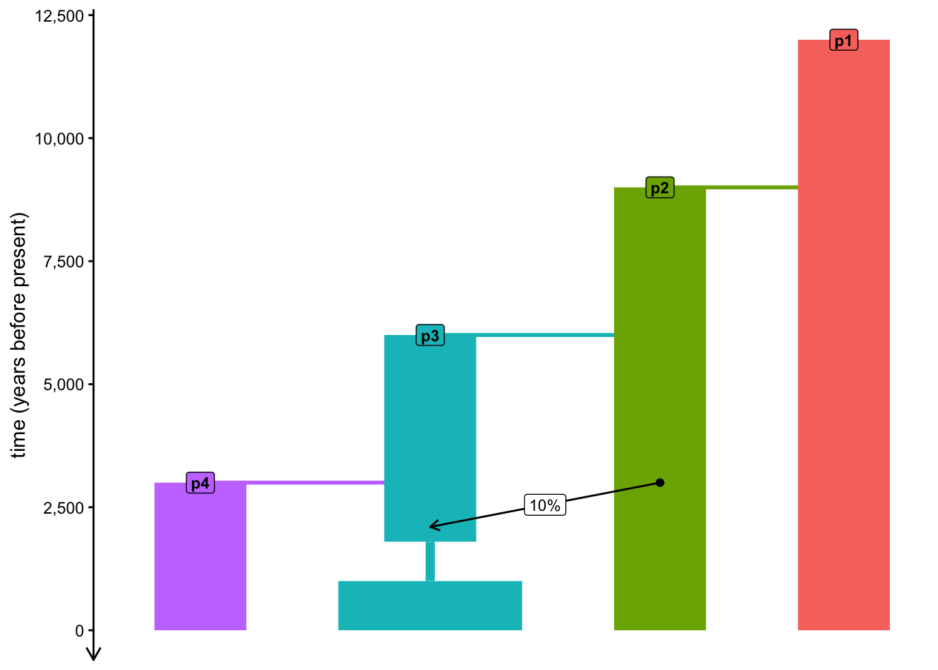
Bonus exercise: Models on disk
Feel free to skip this exercise, unless you managed to run through everything quickly or want to learn a little bit about slendr internals. Knowing a little bit about what’s going on behind the curtain of the software that we take for granted can come in very handy at times.
A very important part of slendr’s approach to modeling is to make simple things be trivially easy. This is largely why expressing even relatively complex models requires so little slendr code compared to the amount of programming needed with other powerful simulators.
Still, sometimes it’s useful to peek behind the curtain and see what exactly is going on inside slendr and how it operates.
Type out the model object in the R console, paying attention to the description of the path where it’s been compiled. Use your operating system’s file browsing program to see what files are hiding in that path. Given the model we’ve programmed so far, pay particular attention to populations.tsv, geneflow.tsv, etc. When you open those files, what format do they have? Can you decipher the meaning of the information they store by comparing it to the code you wrote in your script human_model.R?
What is stored in the files script.py and script.slim? If you know a bit of either Python or SLiM, can you decipher how will slendr (later, as we’ll see) simulate data?