Custom SLiM or Python simulations • demografr

⚠️⚠️⚠️

Note: The demografr R package is still under active development. As a result, its documentation is in a draft stage at best. Typos, inconsistencies, and other issues are unfortunately expected.

⚠️⚠️⚠️️⚠️

By default, demografr uses the slendr simulation framework for defining models and simulating data from them. But what if you need to do inference using your own scripts? Perhaps slendr’s opinionated interface doesn’t allow you to do all that you need to do, such as using some of the powerful simulation features and options of “raw” SLiM or msprime? This vignette explains how you can use any standard SLiM or msprime script which produces a tree sequence file as its output as an engine in a standard demografr inference pipeline.

First, let’s load demografr itself and also slendr (which, in this vignette, will serve only for analyzing simulated tree-sequence data, but not simulations themselves).

library(demografr)
library(slendr)

init_env(quiet = TRUE)

Restrictions on user-defined simulation scripts

In order to be able to use a custom SLiM or msprime script with demografr, the script must conform to a couple of rules:

1. It must be runnable on the command-line as any other command-line script

For an msprime script, this means something like python <your script>.py <command-line arguments>.
For a SLiM script, this means something like slim <command-line arguments> <your script>.slim.

2. It must accept three mandatory arguments with these exact names

sequence_length: the amount of sequence to simulated
recombination_rate: the recombination rate along the simulated sequence (in units of crossovers per basepair pergeneration)
output_path: the path where the simulated tree-sequence object will be saved

For an msprime script, these parameters can be specified via the Python built-in module argparse, and provided on the command-line as --sequence_length <value>, --recombination_rate <value>, and --output_path <path>. In the script itself, if you use the argparse module and have thus the values of provided arguments (for instance) in an args object, you can then refer to these arguments as args.sequence_length, etc.

For a SLiM script, these parameters can be specified via SLiM’s standard way of supplying command-line arguments as -d sequence_length=<value>, -d recombination_rate=<value>, and -d "output_path='<path>'". Importantly, note SLiM’s format of specifying string arguments for the output_path argument. If you need further detail, see Section 20.2 of the SLiM manual. In the script itself, you can then refer to these arguments via constants sequence_length, recombination_rate, and output_path.

3. All model parameters must be provided as additional command-line arguments

You can refer to them in your script as you would to the mandatory arguments as described in the previous section.

A useful check to see whether you script would make a valid engine for a demografr analysis is to run it manually on the command line like this:

python \
  <path to your Python script>                   \
  --sequence_length <number>                     \
  --recombination_rate <number>                  \
  --output_path <path to the output .trees file> \
  <... your model parameters ...>

Or, if you want to run a SLiM-powered ABC, like this:

slim \
  -d sequence_length=<number>                         \
  -d recombination_rate=<number>                      \
  -d "output_path='<path to the output .trees file>'" \
  <... your model parameters ...>

Then, if you get a .trees file, you’re good to go!

Note that mutation rate is not among the list of mandatory parameters for your script. Neutral mutations are taken care of via tree-sequence mutation process after the simulation is finished. If this sounds weird to you, take a look at some tree-sequence-related materials like this.

ABC analysis using custom-defined simulation scripts

Toy problem

Suppose that we intent to use ABC to infer the \(N_e\) of a constant-sized population given that we observed the following value of nucleotide diversity:

observed_diversity

#> # A tibble: 1 × 2
#>   set   diversity
#>   <chr>     <dbl>
#> 1 pop   0.0000198

We want to infer the posterior distribution of \(N_e\) but not via the normal slendr interface (as shown here) but using a simple SLiM or Python script.

We acknowledge that this is a completely trivial example, not really worth spending so much effort on doing an ABC for. The example was chosen because it runs fast and demonstrates all the features of demografr that you would use regardless of the complexity of your model.

Example pure SLiM and msprime script

To demonstrate the requirements 1-3 above in practice, let’s perform ABC using each of those scripts as tree-sequence simulation engines.

Imagine we have the following two scripts which we want to use as simulation engines instead of slendr’s own functions slim() and msprime(). The scripts have only one model parameter, \(N_e\) of the single modelled population. The other parameters are mandatory, just discussed in the previous section.

SLiM script

slim_script <- system.file("examples/custom.slim", package = "demografr")

initialize() {
  initializeTreeSeq();
  initializeMutationRate(0);
  initializeMutationType("m1", 0.5, "f", 0.0);
  initializeGenomicElementType("g1", m1, 1.0);
  initializeGenomicElement(g1, 0, sequence_length - 1);
  initializeRecombinationRate(recombination_rate);
}

1 early() {
  sim.addSubpop("p0", asInteger(Ne));
}

10000 late() {
  sim.treeSeqOutput(output_path); // this call must be present in every script
}

Python script

python_script <- system.file("examples/custom.py", package = "demografr")

import argparse

import msprime

parser = argparse.ArgumentParser()

# mandatory command-line arguments
parser.add_argument("--sequence_length", type=float, required=True)
parser.add_argument("--recombination_rate", type=float, required=True)
parser.add_argument("--output_path", type=str, required=True)

# model parameters
parser.add_argument("--Ne", type=float, required=True)

args = parser.parse_args()

ts = msprime.sim_ancestry(
  samples=round(args.Ne),
  population_size=args.Ne,
  sequence_length=args.sequence_length,
  recombination_rate=args.recombination_rate,
)

ts.dump(args.output_path) # this call must be present in every script

Note that the Python script specifies all model parameters (here, \(N_e\)) and mandatory arguments, via a command-line interface provided by the Python module argparse.

The SLiM script, on the other hand, uses SLiM’s features for command-line specification of parameters and simply refers to each parameter by its symbolic name. No other setup is necessary.

Please also note that given that there are can be discrepancies between values of arguments of some SLiM or Python methods (such as addSubPop of SLiM which expects an integer value for a population size, or the samples argument of msprime.sim_ancestry), and values of parameters sampled from priors by demografr (i.e., \(N_e\) often being a floating-point value after sampling from a continuous prior), you might have to perform explicit type conversion in your custom scripts (such as sim.addSubPop("p0", asInteger(Ne) as above).

Individual ABC components

Apart from the user-defined simulation SLiM and msprime scripts, the components of our toy inference remains the same—we need to define the observed statistics, tree-sequence summary functions, and priors. We don’t need a model function—that will be served by our custom script.

Here are the demografr pipeline components (we won’t be discussing them here because that’s extensively taken care of elsewhere in demografr’s documentation vignettes):

# a single prior parameter
priors <- list(Ne ~ runif(10, 1000))

# a single observed statistic
observed <- list(diversity = observed_diversity)

# a single tree-sequence summary function producing output in the same
# format as the observed statistic table
functions <- list(
  diversity = function(ts) {
    ts_diversity(ts, list(pop = seq(0, 19))) # compute using 20 chromosomes
  }
)

(Note that because our simulated tree sequences won’t be coming with slendr metadata, we have to refer to individuals’ chromosomes using numerical indices rather than slendr symbolic names like we do in all of our other vignettes.)

Simulating a testing tree sequence

As we explained elsewhere, a useful function for developing inference pipelines using demografr is a function simulate_ts(), which normally accepts a slendr model generating function and the model parameters (either given as priors or as a list of named values), and simulates a tree-sequence object. This function (as any other demografr function operating with models) accepts our custom-defined simulation scripts in place of standard slendr models.

For instance, we can simulate a couple of Mb of testing sequence from our msprime script like this:

ts_python <- simulate_ts(
  model = python_script, parameters = list(Ne = 1234),
  sequence_length = 10e6, recombination_rate = 1e-8, mutation_rate = 1e-8
)

(Of course we could’ve plugged in the python_script instead.)

Now we can finally test our little toy tree-sequence summary function, verifying that we can indeed compute the summary statistic we want to:

functions$diversity(ts_python)

#> # A tibble: 1 × 2
#>   set   diversity
#>   <chr>     <dbl>
#> 1 pop   0.0000536

The function works as expected—we have a single population and want to compute nucleotide diversity in the whole population, and this is exactly what we get.

Running an ABC analysis

Having all components of our pipeline set up we should, again, validate everything before we proceed to (potentially very costly) simulations. In the remainder of this vignette we’ll only continue with the Python msprime custom script in order to save some computational time. That said, it’s important to realize that you could use this sort of workflow for any kind of SLiM script, including very elaborate spatial simulations, non-WF models, and all kinds of phenotypic simulations too! Although primarily designed to work with slendr, the demografr package intends to fully support any kind of SLiM or msprime simulation.

Let’s first validate all components of our pipeline:

validate_abc(python_script, priors, functions, observed)

#> ======================================================================
#> Testing sampling of each prior parameter:
#>   * Ne ✅
#> ---------------------------------------------------------------------
#> The model is a custom user-defined msprime script
#> ---------------------------------------------------------------------
#> Simulating tree sequence from the given model... ✅
#> ---------------------------------------------------------------------
#> Computing user-defined summary functions:
#>   * diversity ✅
#> ---------------------------------------------------------------------
#> Checking the format of simulated summary statistics:
#>   * diversity ✅  
#> ======================================================================
#> No issues have been found in the ABC setup!

Looking good! Now let’s first run ABC simulations. Again, note the use of the Python script where we would normally plug in a slendr model function in place of the model argument:

library(future)
plan(multicore, workers = availableCores()) # parallelize across all 96 CPUs

data <- simulate_abc(
  model = python_script, priors, functions, observed, iterations = 1000,
  sequence_length = 1e6, recombination_rate = 1e-8, mutation_rate = 1e-8
)

The total runtime for the ABC simulations was 0 hours 2 minutes 39 seconds parallelized across 96 CPUs.

Once the simulations are finished, we can perform inference of the posterior distribution of the single parameter of our model, \(N_e\):

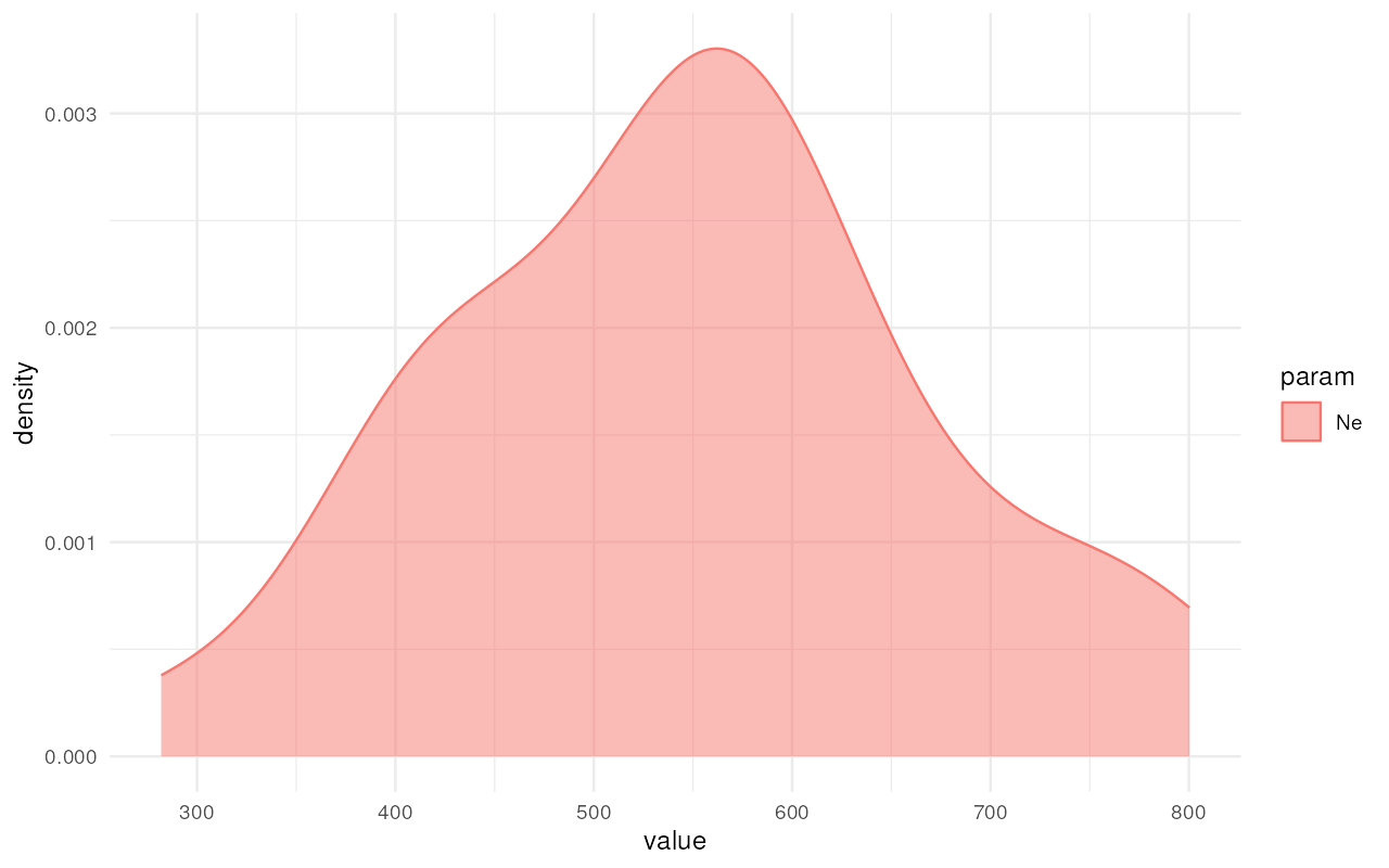
abc <- run_abc(data, engine = "abc", tol = 0.03, method = "neuralnet")

Having done so, we can again look at the summary statistics of the posterior distribution and also plot the results (we’re skipping diagnostics such as posterior predictive checks but you can read more about those here and here):

extract_summary(abc)

#> Warning in density.default(x, weights = weights): Selecting bandwidth *not*
#> using 'weights'

#>                              Ne
#> Min.:                  281.9347
#> Weighted 2.5 % Perc.:  281.9347
#> Weighted Median:       568.4176
#> Weighted Mean:         555.8596
#> Weighted Mode:         571.6191
#> Weighted 97.5 % Perc.: 800.3001
#> Max.:                  800.3001

plot_posterior(abc)